BigSEM User Manual
This is the user manual of BigSEM to show how to conduct SEM with network data and text data. If you want to contribute to its development, please check out our development manual.
- What is BigSEM?
- BigSEM for network data
- SEM with networks - background
- Example datasets
- Node based analysis with network statistics
- Node based analysis with latent space model
- Edge based analysis with edge values
- Edge based analysis with latent space model
- Use of Web App for SEM with Networks
- BigSEM for Text Data
What is BigSEM?
BigSEM is a collection of software programs for conducting SEM analysis with new types of data such as network data and text data.
How to install BigSEM?
BigSEM can be used either locally as R packages or online using our web app.
R Package
We have two R packages in the development stage that can now be installed from GitHub. The packages will be available on CRAN soon. The R package networksem can be used for SEM network analysis and the package TextSEM can be used for text analysis.
## Install the package for network analysis
remotes::install_github("iasnobmatsu/networksem")

## Install the package for text analysis
remotes::install_github("Stan7s/TextSEM")
Web App
To use our web app, go to the website at https://bigsem.psychstat.org/app. Note that you will be prompted to log in as a user. If you don't have an account, you can register one for free.
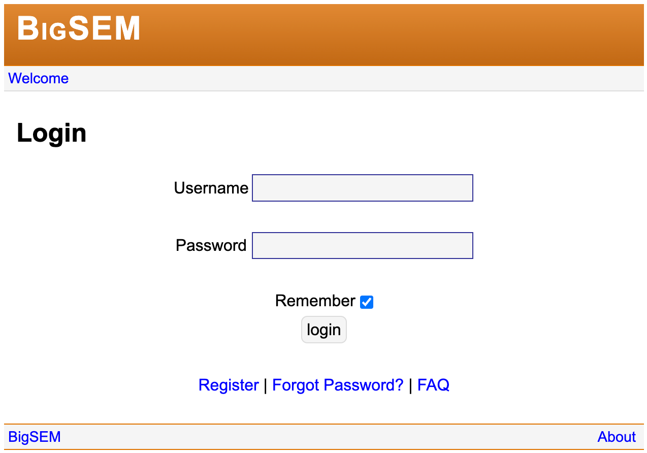
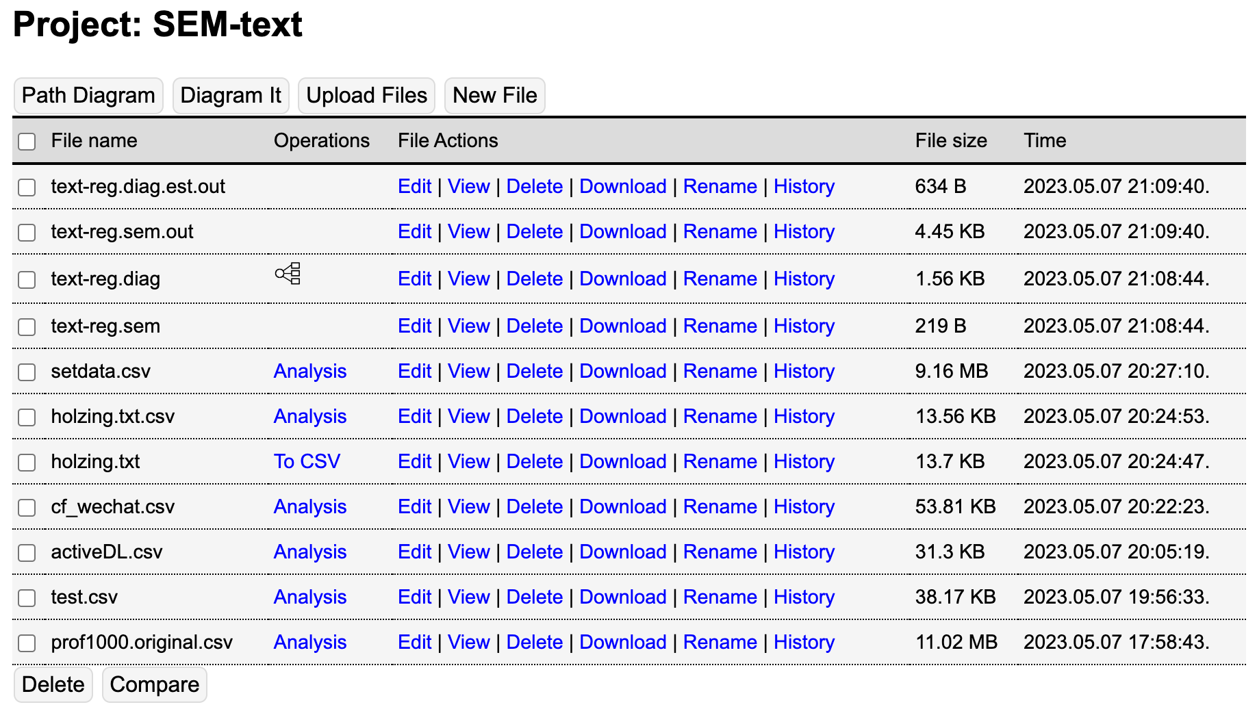
Once logging in our web app, one can create a project and start to conduct the analysis. Note that we manage projects as files. One can upload, create, and delete files within the app.
BigSEM for network data
We will show how to use BigSEM to analyze network data in the SEM framework.
SEM with networks - background
Network data can be integrated into the SEM framework in different ways. We focus on two main approaches here. The first approach extracts the information from a network based on each participant and then use that information as variable(s) in a SEM model. In this method, each participant (node) in the network is the basic unit for analysis. The second approach extracts information from a network based on each relationship present. In this method, each pair of participants or nodes are used as the basic unit for analysis.
In our software, we propose and implement four types of models.
Network nodes as analysis units
In this method, each participant is treated as the basic unit of analysis. Therefore, the sample size is equal the sample size $n$. We use two approaches here: (1) we extract information as network statistics from a network, and (2) we extract information through a latent space model.
Use network statistics
We denote a network through a square adjacency matrix $\mathbf{M}=[m_{ij}]$ with each $m_{ij}$ denoting the connection between subject $i$ and subject $j$. Based on the adjacency matrix, many node-based network statistics can be defined. For example, the statistic degree is a centrality measure that simply counts how many subjects a subject connects to in the network. The statistic betweenness measures the extent to which a subject lies on the paths between other subjects. Subjects with high betweenness influence how the information flows in the network. Both degree and betweenness quantify the importance of a subject in a network. For example, for our friendship network, if a student has a larger degree, he or she is more popular in the network. From a network, we can derive a vector of network statistics for each subject $i$ as $\mathbf{t}_{i}(\mathbf{M})$ .
Because the network statistics are node based, the dimension of the resulting network statistics data will match the non-network data, and they can be combined to be used in SEM as any regular SEM analysis.
Use latent space model
In this approach, each subject assumes a position in a Euclidean space. The distance of two subjects in the latent space is assumed to be related to how likely they are connected in the network. The idea of latent space modeling is similar to that of factor analysis
with a latent factor space and factor scores. Let $\mathbf{z}_{i}$ be a vector of latent positions of subject $i$ in the latent space. For subjects $i$ and $j$, the Euclidean distance between them is:
\begin{equation}
d_{ij}({\bf z}_{i},{\bf z}_{j})=\sqrt{({\bf z}_{i}-{\bf z}_{j})^{t}({\bf z}_{i}-{\bf z}_{j})}=\sqrt{\sum_{d=1}^{D}({z}_{i,d}-{z}_{j,d})^{2}}
\label{eq:distance}
\end{equation}
where $(\cdot)^{t}$ is the transpose of a matrix or vector, $D$ is the dimension of the Euclidean latent space, $\mathbf{z}_{i}=(z_{i,1},z_{i,2},\cdots,z_{i,D})^{t}$ and $\mathbf{z}_{j}=(z_{j,1},z_{j,2},\cdots,z_{j,D})^{t}$ are the latent positions of subjects $i$ and $j$, respectively. With the distance, the latent space model can be written as
\begin{equation}
\begin{cases}
m_{ij} & \sim\text{Bernoulli}(p_{ij})\\
\text{logit}[p(m_{ij})] & =\alpha+\boldsymbol{\beta}'{\bf h}_{ij}-\kappa\times d_{ij}({\bf z}_{i},{\bf z}_{j})
\end{cases}\label{eq:LSM}
\end{equation}
where $\alpha$ is an intercept, ${\bf h}_{ij}$ is a vector of covariates and $\boldsymbol{\beta}$ contains the coefficients of the covariates. Note that the network is assumed to be unweighted here. In our software, following the tradition in network analysis, the coefficient $\kappa$ for $d_{ij}$ is fixed as 1 because $\kappa$ can be rescaled together with the distance (Hoff et al., 2002). Therefore, the closer of two subjects are in the latent space, the higher the probability is for them to be connected after controlling the covariates in the model.
Here, we adapt and extend the latent space model to have the form shown below:
\begin{equation}
\begin{cases}
E(m_{ij}) & =\mu_{ij}\\
g(\mu_{ij}) & =\alpha-d_{ij}({\bf z}_{i},{\bf z}_{j})
\end{cases}\label{eq:SEM-LSM}
\end{equation}
where $g$ is a link function. First, we assume the connection between two subjects is solely explained by the latent space. Second, we relax the requirement of the Bernoulli distribution to use any exponential family of distributions. Using this model, we can extract information from a network. The idea is similar to principal component analysis. In our model, the latent positions will be used along with non-network variables in the SEM framework.
Network edges as analysis units
Another approach we take is to use edges as the unit of interest. In this case, non-network data are reformatted for analysis to be based on pairs of individuals. In this case, given a non-network covariate $c$, we define $c_{ij} = f(c_i, c_j)$, where $c_i$ and $c_j$ are the covariate values for individual $i$ and individual $j$. The function $f$ can be chosen according to the purpose of the analysis. For example, $c_{ij}$ can be the average of $c_i$ and $c_j$, or it can be the difference. Then, these pairwise non-network variables can be used as either endogenous or exogenous variables.
Use network statistics
Similar as in the node-based framework, in the edge-based framework, network statistics that can be obtained free from assuming underlying models to the social network can be used in SEM. The network statistics are constructed based on each pairs of subjects. For example, the shortest path length between each pair of nodes can be used as the edge-based network statistics.
Use latent space model
The latent space modeling approach can also be used when using a pair of subjects as the unit of analysis. In this case, the latent distance between two subjects $d_{ij}(z_i, z_j)$ can be used in SEM instead of the latent positions $z_i$ and $z_j$.
Example datasets
We will use several datasets to illustrate the use of our software.
Friendship Network Data
In this dataset, information on friendship network, alcohol use, smoking, the big five personality traits, and academic performance among college students is collected for three years in 2017, 2018, and 2019. The participants were undergraduate students and the sample size is $N = 165$. There were about an equal number of male and female students (45% vs. 55%) in the sample. The average age of the students was 21.64 ($SD$ = 0.85). The average GPA of the students was about 3.273 ($SD$ = 0.53) out of 5.
Information on two social networks was collected. First, each student was presented a list of all the students in the study and was asked to report his/her acquaintanceship with everyone else on the list, on a Likert scale of 0 to 4. Second, each student was asked to report whether the students on the list were their WeChat friends or not (WeChat is a popular social network platform in China). Therefore, there are two friendship networks: the first one is a real-life weighted acquaintanceship network (referred to as the acquaintance network) and the second one is a virtual unweighted social media network (referred to as the WeChat network). The two networks together can be viewed as a multiplex network. Data on personality, happiness, depression, and loneliness were also collected.
Attorney Network Data
The second dataset includes the cowork and advice network dataset from 71 attorneys from a law firm called SG&R in 1988. The dataset is available from the SIENA website. The first wave of network data will be used in the analysis in the current tutorial. The cowork information is collected by asking the company employees to select people who have worked on the same case with them. Additionally, information on an advice network is collected via asking respondents who they seek advice from at work. Several non-network attributes are collected alongside with the networks. From those, the office one works at (i.e., Boston, Hartford, and Providence) and years with the firm will be used for analysis.
Florentine Marriage Data
The dataset is from Breiger and Pattison (1986), where the social network indicates marriage alliances, and the non-network variables include (1) wealth, each family’s net wealth in 1427 (in thousands of lira); (2) priorates, the number of priorates (seats on the civic council) held between 1282- 1344; and (3) totalties, the total number of business or marriage ties in the total dataset of 116 families.
Node based analysis with network statistics
The function sem.net can be used to fit a SEM model with network data using node statistics as variables. User-specified network statistics will be calculated and used as variables instead of the networks themselves in the SEM.
The following choices of network statistics can be used:
degree: Degree is a centrality measure that counts actors/nodes a specific node is connected to.betweenness: Betweenness is a centrality measure that counts how many shortest path an actor is crossed by through a random choice. It measures how much an individual control the spread of information.closeness: Closeness is a measure of how efficiently a node spreads information and can be calculated by the average inverse distance from a node to all other nodes.evcent: The eigenvector centrality is a measure of transitive influence of each node, meaning that a node with high eigenvector centrality tends to connect with other nodes with high eigenvector centrality (Ruhnau, 2000).stresscent: Stress centrality is similar to betweenness centrality as it also measures the control of spread. However, while betweenness centrality measures through a random fraction of shortest paths, stress centrality takes into account all shortest paths (Szczepanski et al., 2012).infocent: Information centrality is defined as the reduction in network efficiency if a target node is removed. It is a measure of node effectiveness in spreading information (Latora and Marchiori, 2007).ivi: Integrated value of influence is a measure that combines different centrality measures (Salavaty et al., 2020a)hubeness.score: Hubeness score is a component of IVI and measures a node’s influence in its surrounding environment.spreading.score: Spreading score is another component of IVI and measures a node’s spreading potential.clusterRank: Cluster rank is a measure of clustering that takes into account a node, its neighbors, and their clustering coefficients.
Simulated Data Example
To begin with, a random simulated dataset can be used to demonstrate the usage of the node-based network statistics approach. The code below generate a simulated network net with four non-network covariates x1 - x4 which loads on two latent variables lv1, lv2.
set.seed(100)
nsamp = 100 # sample size
net <- ifelse(matrix(rnorm(nsamp^2), nsamp, nsamp) > 1, 1, 0) # simulate network
mean(net) # density of simulated network

# simulate non-network variables
lv1 <- rnorm(nsamp)
lv2 <- rnorm(nsamp)
nonnet <- data.frame(x1 = lv1*0.5 + rnorm(nsamp),
                     x2 = lv1*0.8 + rnorm(nsamp),
                     x3 = lv2*0.5 + rnorm(nsamp),
                     x4 = lv2*0.8 + rnorm(nsamp))
With the simulated data, we can define a model string with lavaan syntax that specifies the measurement model as well as the relationship between the network and the non-network variables. In this case, we are using net as a mediator between the two latent variables. Since data are generated randomly, the effects should be small overall.
model <-'
  lv1 =~ x1 + x2
  lv2 =~ x3 + x4
  net ~ lv2
  lv1 ~ net + lv2
'
Arguments passed to the sem.net function includes the model, the dataset, and the network statistics of interest. Note that data here should be a list with two elements, one being the named list of all network variables and one being the dataframe containing non-network variables. A summary function can be used to look at the output, and the function path.networksem can be used to look at mediation effects.
data = list(network = list(net = net), nonnetwork = nonnet)
set.seed(100)
res <- sem.net(model = model, data = data, netstats = c('degree'))
summary(res)
path.networksem(res, "lv2", c("net.degree"), "lv1")
The output of should look like the following.
> summary(res)
The SEM output:
lavaan 0.6.15 ended normally after 54 iterations

  Estimator                                         ML
  Optimization method                           NLMINB
  Number of model parameters                        12

  Number of observations                           100

Model Test User Model:

  Test statistic                                 1.230
  Degrees of freedom                                 3
  P-value (Chi-square)                           0.746

Model Test Baseline Model:

  Test statistic                                24.987
  Degrees of freedom                                10
  P-value                                        0.005

User Model versus Baseline Model:

  Comparative Fit Index (CFI)                    1.000
  Tucker-Lewis Index (TLI)                       1.394

Loglikelihood and Information Criteria:

  Loglikelihood user model (H0)               -913.294
  Loglikelihood unrestricted model (H1)       -912.679

  Akaike (AIC)                                1850.588
  Bayesian (BIC)                              1881.850
  Sample-size adjusted Bayesian (SABIC)       1843.951

Root Mean Square Error of Approximation:

  RMSEA                                          0.000
  90 Percent confidence interval - lower         0.000
  90 Percent confidence interval - upper         0.118
  P-value H_0: RMSEA <= 0.050                    0.810
  P-value H_0: RMSEA >= 0.080                    0.120

Standardized Root Mean Square Residual:

  SRMR                                           0.026

Parameter Estimates:

  Standard errors                             Standard
  Information                                 Expected
  Information saturated (h1) model          Structured

Latent Variables:
                   Estimate  Std.Err  z-value  P(>|z|)
  lv2 =~
    x4                1.000
    x3                2.035    2.162    0.941    0.347
  lv1 =~
    x2                1.000
    x1                1.056    0.789    1.338    0.181

Regressions:
                   Estimate  Std.Err  z-value  P(>|z|)
  lv1 ~
    lv2              -0.441    0.300   -1.470    0.142
  net.degree ~
    lv2              -0.934    1.163   -0.804    0.422
  lv1 ~
    net.degree       -0.011    0.020   -0.569    0.569

Variances:
                   Estimate  Std.Err  z-value  P(>|z|)
   .x4                1.350    0.293    4.603    0.000
   .x3                0.215    0.923    0.233    0.816
   .x2                1.002    0.299    3.357    0.001
   .x1                1.047    0.328    3.190    0.001
   .net.degree       22.292    3.164    7.046    0.000
    lv2               0.214    0.249    0.860    0.390
   .lv1               0.302    0.264    1.142    0.253

> path.networksem(res, "lv2", c("net.degree"), "lv1")
  predictor   mediator outcome     apath       bpath   indirect indirect_se  indirect_z
1       lv2 net.degree     lv1 -0.934393 -0.01126621 0.01052707    1.086552 0.009688509
Empirical Data Example
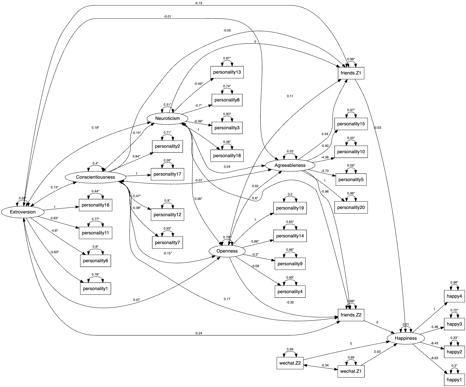
Using the friendship network data, a model with 5 personality traits and two networks' effect on happiness can be fitted using the code below. In this case, degree, betweenness, closeness are used as network statistics.
# load data
load("data/cf_data_book.RData")  ## load the list cf_data

## data - non-network variables
non_network <- as.data.frame(cf_data$cf_nodal_cov)
dim(non_network)

## network - network variables (friends network and wechat network)
## note that the names of the networks are used in model specification
network <- list()
network$friends <- cf_data$cf_friend_network
network$wechat <- cf_data$cf_wetchat_network

model <-'
  Extroversion =~ personality1 + personality6
                + personality11 + personality16
  Conscientiousness =~ personality2 + personality7
                + personality12 + personality17
  Neuroticism  =~ personality3 + personality8
                + personality13 + personality18
  Openness =~ personality4 + personality9
                + personality14 + personality19
  Agreeableness =~ personality5 + personality10 +
                personality15 + personality20
  Happiness =~ happy1 + happy2 + happy3 + happy4
  friends ~ Extroversion + Conscientiousness + Neuroticism +
  Openness + Agreeableness
  Happiness ~ friends + wechat
'

## run sem.net
data = list(
  nonnetwork = non_network,
  network = network
)

set.seed(100)
res <- sem.net(model=model, data=data,
               netstats=c("degree", "betweenness", "closeness"),
               netstats.rescale = T,
               netstats.options=list("degree"=list("cmode"="freeman")))

## results
summary(res)
The output of the analysis is given below:
lavaan 0.6-18 ended normally after 453 iterations

  Estimator                                         ML
  Optimization method                           NLMINB
  Number of model parameters                        82

  Number of observations                           165

Model Test User Model:

  Test statistic                               844.769
  Degrees of freedom                               377
  P-value (Chi-square)                           0.000

Model Test Baseline Model:

  Test statistic                              1795.826
  Degrees of freedom                               432
  P-value                                        0.000

User Model versus Baseline Model:

  Comparative Fit Index (CFI)                    0.657
  Tucker-Lewis Index (TLI)                       0.607

Loglikelihood and Information Criteria:

  Loglikelihood user model (H0)              -6286.542
  Loglikelihood unrestricted model (H1)      -5864.157

  Akaike (AIC)                               12737.084
  Bayesian (BIC)                             12991.771
  Sample-size adjusted Bayesian (SABIC)      12732.159

Root Mean Square Error of Approximation:

  RMSEA                                          0.087
  90 Percent confidence interval - lower         0.079
  90 Percent confidence interval - upper         0.095
  P-value H_0: RMSEA <= 0.050                    0.000
  P-value H_0: RMSEA >= 0.080                    0.922

Standardized Root Mean Square Residual:

  SRMR                                           0.116

Parameter Estimates:

  Standard errors                             Standard
  Information                                 Expected
  Information saturated (h1) model          Structured

Latent Variables:
                       Estimate  Std.Err  z-value  P(>|z|)
  Happiness =~
    happy4                1.000
    happy3               -4.283    3.684   -1.162    0.245
    happy2               -6.682    5.698   -1.173    0.241
    happy1               -6.955    5.932   -1.172    0.241
  Agreeableness =~
    personality20         1.000
    personality15        -1.200    0.905   -1.326    0.185
    personality10        -4.293    2.506   -1.713    0.087
    personality5         -4.462    2.606   -1.712    0.087
  Openness =~
    personality19         1.000
    personality14         0.784    0.165    4.748    0.000
    personality9         -0.224    0.106   -2.110    0.035
    personality4         -0.097    0.108   -0.898    0.369
  Neuroticism =~
    personality18         1.000
    personality13        -0.532    0.148   -3.603    0.000
    personality8         -0.808    0.176   -4.602    0.000
    personality3         -0.378    0.136   -2.778    0.005
  Conscientiousness =~
    personality17         1.000
    personality12        -0.693    0.214   -3.235    0.001
    personality7         -0.508    0.219   -2.319    0.020
    personality2          1.108    0.265    4.187    0.000
  Extroversion =~
    personality16         1.000
    personality11         0.609    0.136    4.493    0.000
    personality6         -0.508    0.123   -4.116    0.000
    personality1         -0.521    0.119   -4.377    0.000

Regressions:
                        Estimate  Std.Err  z-value  P(>|z|)
  friends.degree ~
    Extroversion           2.355    1.126    2.091    0.037
  friends.betweenness ~
    Extroversion           2.119    1.048    2.023    0.043
  friends.closeness ~
    Extroversion           2.175    1.026    2.119    0.034
  friends.degree ~
    Conscientisnss        -8.447    5.060   -1.670    0.095
  friends.betweenness ~
    Conscientisnss        -7.827    4.706   -1.663    0.096
  friends.closeness ~
    Conscientisnss        -7.720    4.609   -1.675    0.094
  friends.degree ~
    Neuroticism           -1.282    1.364   -0.940    0.347
  friends.betweenness ~
    Neuroticism           -1.252    1.272   -0.985    0.325
  friends.closeness ~
    Neuroticism           -1.324    1.248   -1.061    0.289
  friends.degree ~
    Openness              -1.355    1.483   -0.914    0.361
  friends.betweenness ~
    Openness              -1.204    1.377   -0.875    0.382
  friends.closeness ~
    Openness              -1.162    1.348   -0.862    0.389
  friends.degree ~
    Agreeableness        -16.541   15.253   -1.084    0.278
  friends.betweenness ~
    Agreeableness        -15.697   14.299   -1.098    0.272
  friends.closeness ~
    Agreeableness        -14.400   13.668   -1.054    0.292
  Happiness ~
    friends.degree        -0.047    0.051   -0.931    0.352
    frinds.btwnnss         0.007    0.025    0.292    0.771
    friends.clsnss         0.062    0.059    1.045    0.296
    wechat.degree          0.013    0.037    0.351    0.725
    wechat.btwnnss         0.050    0.049    1.027    0.305
    wechat.closnss        -0.064    0.060   -1.063    0.288

Covariances:
                       Estimate  Std.Err  z-value  P(>|z|)
  Agreeableness ~~
    Openness              0.015    0.018    0.866    0.386
    Neuroticism           0.043    0.029    1.479    0.139
    Conscientisnss       -0.072    0.044   -1.643    0.100
    Extroversion         -0.011    0.020   -0.554    0.579
  Openness ~~
    Neuroticism           0.330    0.074    4.446    0.000
    Conscientisnss       -0.166    0.059   -2.806    0.005
    Extroversion          0.089    0.080    1.111    0.266
  Neuroticism ~~
    Conscientisnss       -0.153    0.058   -2.648    0.008
    Extroversion          0.212    0.082    2.588    0.010
  Conscientiousness ~~
    Extroversion          0.174    0.070    2.490    0.013

Variances:
                   Estimate  Std.Err  z-value  P(>|z|)
   .happy4            2.702    0.298    9.066    0.000
   .happy3            1.226    0.147    8.353    0.000
   .happy2            0.577    0.139    4.146    0.000
   .happy1            0.507    0.145    3.496    0.000
   .personality20     1.107    0.123    8.979    0.000
   .personality15     1.195    0.134    8.945    0.000
   .personality10     0.617    0.115    5.359    0.000
   .personality5      0.742    0.130    5.705    0.000
   .personality19     0.244    0.125    1.948    0.051
   .personality14     0.680    0.107    6.372    0.000
   .personality9      0.854    0.095    8.982    0.000
   .personality4      0.963    0.106    9.067    0.000
   .personality18     0.498    0.104    4.790    0.000
   .personality13     0.920    0.109    8.469    0.000
   .personality8      0.965    0.125    7.694    0.000
   .personality3      0.893    0.102    8.768    0.000
   .personality17     0.707    0.088    8.051    0.000
   .personality12     1.042    0.119    8.753    0.000
   .personality7      1.286    0.144    8.940    0.000
   .personality2      1.193    0.143    8.337    0.000
   .personality16     0.595    0.152    3.917    0.000
   .personality11     1.125    0.140    8.023    0.000
   .personality6      1.043    0.126    8.305    0.000
   .personality1      0.902    0.111    8.122    0.000
   .friends.degree    0.074    0.026    2.872    0.004
   .frinds.btwnnss    0.236    0.034    6.912    0.000
   .friends.clsnss    0.170    0.029    5.849    0.000
   .Happiness         0.024    0.040    0.587    0.557
    Agreeableness     0.030    0.034    0.874    0.382
    Openness          0.652    0.155    4.209    0.000
    Neuroticism       0.495    0.129    3.822    0.000
    Conscientisnss    0.248    0.082    3.038    0.002
    Extroversion      0.843    0.199    4.240    0.000
The multiple mediation from Agreeableness to friendship network to Happiness can be calculated using the following code.
> path.networksem(res, 'Agreeableness',
                        c('friends.degree', 'friends.betweenness', 'friends.closeness'),
                        'Happiness')

      predictor            mediator   outcome     apath        bpath   indirect
1 Agreeableness      friends.degree Happiness -16.54130 -0.047133471  0.7796491
2 Agreeableness friends.betweenness Happiness -15.69767  0.007403778 -0.1162220
3 Agreeableness   friends.closeness Happiness -14.40081  0.061957757 -0.8922416
  indirect_se    indirect_z
1    252.3110  0.0030900323
2    224.4727 -0.0005177557
3    196.8378 -0.0045328765
The model used here is shown in the diagram below. The model has the following features:
- We use two networks - friendship and WeChat networks.
- Three network statistics are used - degree, closeness, and betweenness.
- Friendship network is used as mediators.

Node based analysis with latent space model
The node-based latent space model approach calculates latent positions of the networks, and use them in the SEM analysis along with non-network variables.
Simulated Data Example
To begin with, a random simulated dataset can be used to demonstrate the usage of the node-based network statistics approach. The code below generate a simulated network net with four non-network covariates x1 - x4 which loads on two latent variables lv1, lv2.
set.seed(10)
nsamp = 50
net <- ifelse(matrix(rnorm(nsamp^2), nsamp, nsamp) > 1, 1, 0)
mean(net) # density of simulated network
lv1 <- rnorm(nsamp)
lv2 <- rnorm(nsamp)
nonnet <- data.frame(x1 = lv1*0.5 + rnorm(nsamp),
                     x2 = lv1*0.8 + rnorm(nsamp),
                     x3 = lv2*0.5 + rnorm(nsamp),
                     x4 = lv2*0.8 + rnorm(nsamp))
With the simulated data, we can define a model string with lavaan syntax that specifies the measurement model as well as the relationship between the network and the non-network variables. In this case, we are using net as a mediator between the two latent variables. Since data are generated randomly, the effects should be small overall.
model <-'
  lv1 =~ x1 + x2
  lv2 =~ x3 + x4
  net ~ lv2
  lv1 ~ net + lv2
'
Arguments passed to the sem.net.lsm function includes the model, the dataset, and the number of latent dimensions. Note that data here should be a list with two elements, one being the named list of all network variables and one being the dataframe containing non-network variables. A summary function can be used to look at the output, and the function path.networksem can be used to look at mediation effects across the two latent dimensions.
data = list(network = list(net = net), nonnetwork = nonnet)
set.seed(100)
res <- sem.net.lsm(model = model, data = data, latent.dim = 2)
summary(res)
path.networksem(res, 'lv2', c('net.Z1', 'net.Z2'), 'lv1')
The output looks like the following.
> summary(res)
Model Fit InformationSEM Test statistics:  3.771276 on 6 df with p-value:  0.7075962
NOTE: It is not certain whether it is appropriate to use latentnet's BIC to select latent space dimension, whether or not to include actor-specific random effects, and to compare clustered models with the unclustered model.
network 1 LSM BIC:  2242.696
========================================
========================================

The SEM output:
lavaan 0.6.15 ended normally after 117 iterations

  Estimator                                         ML
  Optimization method                           NLMINB
  Number of model parameters                        15

  Number of observations                            50

Model Test User Model:

  Test statistic                                 3.771
  Degrees of freedom                                 6
  P-value (Chi-square)                           0.708

Model Test Baseline Model:

  Test statistic                                34.438
  Degrees of freedom                                15
  P-value                                        0.003

User Model versus Baseline Model:

  Comparative Fit Index (CFI)                    1.000
  Tucker-Lewis Index (TLI)                       1.287

Loglikelihood and Information Criteria:

  Loglikelihood user model (H0)               -434.447
  Loglikelihood unrestricted model (H1)       -432.561

  Akaike (AIC)                                 898.893
  Bayesian (BIC)                               927.574
  Sample-size adjusted Bayesian (SABIC)        880.491

Root Mean Square Error of Approximation:

  RMSEA                                          0.000
  90 Percent confidence interval - lower         0.000
  90 Percent confidence interval - upper         0.138
  P-value H_0: RMSEA <= 0.050                    0.765
  P-value H_0: RMSEA >= 0.080                    0.165

Standardized Root Mean Square Residual:

  SRMR                                           0.062

Parameter Estimates:

  Standard errors                             Standard
  Information                                 Expected
  Information saturated (h1) model          Structured

Latent Variables:
                   Estimate  Std.Err  z-value  P(>|z|)
  lv2 =~
    x4                1.000
    x3                4.622    6.418    0.720    0.471
  lv1 =~
    x2                1.000
    x1               -0.088    0.271   -0.326    0.744

Regressions:
                   Estimate  Std.Err  z-value  P(>|z|)
  lv1 ~
    lv2              -0.984    0.432   -2.279    0.023
  net.Z1 ~
    lv2              -0.159    0.207   -0.765    0.444
  net.Z2 ~
    lv2               0.208    0.257    0.809    0.418
  lv1 ~
    net.Z1           -0.215    0.169   -1.277    0.202
    net.Z2            0.255    0.138    1.850    0.064

Variances:
                   Estimate  Std.Err  z-value  P(>|z|)
   .x4                1.947    0.425    4.581    0.000
   .x3               -1.587    3.655   -0.434    0.664
   .x2                2.927    6.822    0.429    0.668
   .x1                1.345    0.274    4.906    0.000
   .net.Z1            0.624    0.124    5.012    0.000
   .net.Z2            0.950    0.189    5.013    0.000
    lv2               0.139    0.227    0.612    0.541
   .lv1              -1.984    6.796   -0.292    0.770

The LSM output:

==========================
Summary of model fit
==========================

Formula:   network::network(data$network[[latent.network[i]]]) ~ euclidean(d = latent.dim)
<environment: 0x7fc43202a550>
Attribute: edges
Model:     Bernoulli
MCMC sample of size 4000, draws are 10 iterations apart, after burnin of 10000 iterations.
Covariate coefficients posterior means:
            Estimate     2.5% 97.5% 2*min(Pr(>0),Pr(<0))
(Intercept) -0.18777 -0.42332  0.05               0.1175

Overall BIC:        2242.696
Likelihood BIC:     2107.714
Latent space/clustering BIC:     134.9814

Covariate coefficients MKL:
              Estimate
(Intercept) -0.8639125


> path.networksem(res, 'lv2', c('net.Z1', 'net.Z2'), 'lv1')
  predictor mediator outcome      apath      bpath   indirect
1       lv2   net.Z1     lv1 -0.1587188 -0.2154100 0.03418961
2       lv2   net.Z2     lv1  0.2081154  0.2547222 0.05301162
  indirect_se indirect_z
1  0.04030792  0.8482108
2  0.05368411  0.9874733
Empirical Data Example
We fit the same model on the friendship and WeChat networks from the network statistics approach using the LSM approach. Under this approach, the latent positions take the roles of the network statistics but the model string can stay the same.
model <-'
  Extroversion =~ personality1 + personality6
                + personality11 + personality16
  Conscientiousness =~ personality2 + personality7
                + personality12 + personality17
  Neuroticism  =~ personality3 + personality8
                + personality13 + personality18
  Openness =~ personality4 + personality9
                + personality14 + personality19
  Agreeableness =~ personality5 + personality10 +
                personality15 + personality20
  Happiness =~ happy1 + happy2 + happy3 + happy4
  friends ~ Extroversion + Conscientiousness + Neuroticism +
  Openness + Agreeableness
  Happiness ~ friends + wechat
'
To fit the model, the sem.net.lsm() function is used. The argument latent.dim should be used to denote the number of latent dimensions to be used in estimating the LSM. A random seed can be set to ensure reproduction of the results, and the argument data.scale = T is used so the scale of the latent positions and the non-network variables are not too different.
data = list(network=network, nonnetwork=non_network)
set.seed(100)
res <- sem.net.lsm(model=model,data=data, latent.dim = 2, data.rescale = T)
For SEM with latent positions, the estimation is again a two-stage process. First, a latent space model with no covariates is used to estimate latent positions through the latentnet R package. The resulting latent positions are then be extracted and compiled into the same dataset as the non-network variables such as the Big Five personality items and the happiness score items, which are then inputted into lavaan to be estimated in the SEM framework. We could again use res$data to access the restructured data with latent positions, and res$model to access the modified model string. The output of sem.net.lsm() has two components in res$estimates - res$estimates$sem.es for lavaan SEM results and res$estimates$lsm.es for latentnet LSM results.
The output of the analysis is given below:
> summary(res)
Model Fit InformationSEM Test statistics:  947.953 on 329 df with p-value:  0
network 1 LSM BIC:  15760.02
network 2 LSM BIC:  15517.77
========================================
========================================

The SEM output:
lavaan 0.6.15 ended normally after 147 iterations

  Estimator                                         ML
  Optimization method                           NLMINB
  Number of model parameters                        74

  Number of observations                           165

Model Test User Model:

  Test statistic                               947.953
  Degrees of freedom                               329
  P-value (Chi-square)                           0.000

Model Test Baseline Model:

  Test statistic                              1448.277
  Degrees of freedom                               377
  P-value                                        0.000

User Model versus Baseline Model:

  Comparative Fit Index (CFI)                    0.422
  Tucker-Lewis Index (TLI)                       0.338

Loglikelihood and Information Criteria:

  Loglikelihood user model (H0)              -5824.045
  Loglikelihood unrestricted model (H1)      -5350.068

  Akaike (AIC)                               11796.089
  Bayesian (BIC)                             12025.929
  Sample-size adjusted Bayesian (SABIC)      11791.645

Root Mean Square Error of Approximation:

  RMSEA                                          0.107
  90 Percent confidence interval - lower         0.099
  90 Percent confidence interval - upper         0.115
  P-value H_0: RMSEA <= 0.050                    0.000
  P-value H_0: RMSEA >= 0.080                    1.000

Standardized Root Mean Square Residual:

  SRMR                                           0.119

Parameter Estimates:

  Standard errors                             Standard
  Information                                 Expected
  Information saturated (h1) model          Structured

Latent Variables:
                       Estimate  Std.Err  z-value  P(>|z|)
  Happiness =~
    happy4                1.000
    happy3               -5.462    4.485   -1.218    0.223
    happy2               -8.435    6.866   -1.229    0.219
    happy1               -8.634    7.029   -1.228    0.219
  Agreeableness =~
    personality20         1.000
    personality15        -0.915    0.722   -1.267    0.205
    personality10        -4.359    2.395   -1.820    0.069
    personality5         -3.726    2.043   -1.824    0.068
  Openness =~
    personality19         1.000
    personality14         0.658    0.144    4.571    0.000
    personality9         -0.201    0.100   -2.004    0.045
    personality4         -0.085    0.097   -0.873    0.383
  Neuroticism =~
    personality18         1.000
    personality13        -0.492    0.139   -3.529    0.000
    personality8         -0.701    0.151   -4.651    0.000
    personality3         -0.359    0.135   -2.664    0.008
  Conscientiousness =~
    personality17         1.000
    personality12        -0.475    0.163   -2.911    0.004
    personality7         -0.383    0.159   -2.412    0.016
    personality2          0.843    0.193    4.378    0.000
  Extroversion =~
    personality16         1.000
    personality11         0.632    0.151    4.181    0.000
    personality6         -0.597    0.148   -4.038    0.000
    personality1         -0.629    0.151   -4.170    0.000

Regressions:
                   Estimate  Std.Err  z-value  P(>|z|)
  friends.Z1 ~
    Extroversion     -0.150    0.179   -0.838    0.402
  friends.Z2 ~
    Extroversion     -0.238    0.199   -1.192    0.233
  friends.Z1 ~
    Conscientisnss   -0.047    0.327   -0.144    0.885
  friends.Z2 ~
    Conscientisnss    0.166    0.347    0.480    0.631
  friends.Z1 ~
    Neuroticism      -0.001    0.234   -0.006    0.995
  friends.Z2 ~
    Neuroticism       0.600    0.303    1.982    0.048
  friends.Z1 ~
    Openness          0.109    0.144    0.756    0.450
  friends.Z2 ~
    Openness         -0.321    0.179   -1.794    0.073
  friends.Z1 ~
    Agreeableness     0.335    1.023    0.328    0.743
  friends.Z2 ~
    Agreeableness    -0.957    1.176   -0.814    0.416
  Happiness ~
    friends.Z1       -0.029    0.025   -1.165    0.244
    friends.Z2       -0.003    0.009   -0.394    0.693
    wechat.Z1         0.027    0.024    1.146    0.252
    wechat.Z2        -0.002    0.009   -0.192    0.848

Covariances:
                       Estimate  Std.Err  z-value  P(>|z|)
  Agreeableness ~~
    Openness              0.018    0.019    0.965    0.334
    Neuroticism           0.041    0.027    1.538    0.124
    Conscientisnss       -0.072    0.041   -1.727    0.084
    Extroversion         -0.009    0.015   -0.553    0.580
  Openness ~~
    Neuroticism           0.365    0.079    4.596    0.000
    Conscientisnss       -0.152    0.068   -2.233    0.026
    Extroversion          0.074    0.070    1.063    0.288
  Neuroticism ~~
    Conscientisnss       -0.153    0.064   -2.391    0.017
    Extroversion          0.177    0.068    2.605    0.009
  Conscientiousness ~~
    Extroversion          0.130    0.063    2.073    0.038

Variances:
                   Estimate  Std.Err  z-value  P(>|z|)
   .happy4            0.985    0.109    9.065    0.000
   .happy3            0.716    0.086    8.332    0.000
   .happy2            0.332    0.080    4.141    0.000
   .happy1            0.300    0.082    3.678    0.000
   .personality20     0.965    0.108    8.968    0.000
   .personality15     0.969    0.108    8.987    0.000
   .personality10     0.436    0.116    3.773    0.000
   .personality5      0.586    0.101    5.806    0.000
   .personality19     0.205    0.154    1.326    0.185
   .personality14     0.652    0.098    6.662    0.000
   .personality9      0.962    0.107    9.013    0.000
   .personality4      0.988    0.109    9.072    0.000
   .personality18     0.485    0.105    4.635    0.000
   .personality13     0.871    0.102    8.529    0.000
   .personality8      0.744    0.096    7.720    0.000
   .personality3      0.928    0.105    8.809    0.000
   .personality17     0.591    0.106    5.555    0.000
   .personality12     0.903    0.105    8.600    0.000
   .personality7      0.935    0.106    8.781    0.000
   .personality2      0.708    0.100    7.046    0.000
   .personality16     0.443    0.116    3.831    0.000
   .personality11     0.774    0.099    7.796    0.000
   .personality6      0.797    0.100    7.983    0.000
   .personality1      0.776    0.099    7.813    0.000
   .friends.Z1        0.963    0.107    8.984    0.000
   .friends.Z2        0.881    0.118    7.497    0.000
   .Happiness         0.009    0.015    0.615    0.539
    Agreeableness     0.029    0.031    0.934    0.350
    Openness          0.789    0.186    4.234    0.000
    Neuroticism       0.509    0.131    3.880    0.000
    Conscientisnss    0.403    0.122    3.310    0.001
    Extroversion      0.551    0.143    3.842    0.000

The LSM output:

==========================
Summary of model fit
==========================

Formula:   network::network(data$network[[latent.network[i]]]) ~ euclidean(d = latent.dim)
<environment: 0x7fc412d34470>
Attribute: edges
Model:     Bernoulli
MCMC sample of size 4000, draws are 10 iterations apart, after burnin of 10000 iterations.
Covariate coefficients posterior means:
            Estimate   2.5%  97.5% 2*min(Pr(>0),Pr(<0))
(Intercept)   2.6130 2.5054 2.7225            < 2.2e-16 ***
---
Signif. codes:  0 ‘***’ 0.001 ‘**’ 0.01 ‘*’ 0.05 ‘.’ 0.1 ‘ ’ 1

Overall BIC:        15760.02
Likelihood BIC:     14056.24
Latent space/clustering BIC:     1703.784

Covariate coefficients MKL:
            Estimate
(Intercept) 2.426421


==========================
Summary of model fit
==========================

Formula:   network::network(data$network[[latent.network[i]]]) ~ euclidean(d = latent.dim)
<environment: 0x7fc412d34470>
Attribute: edges
Model:     Bernoulli
MCMC sample of size 4000, draws are 10 iterations apart, after burnin of 10000 iterations.
Covariate coefficients posterior means:
            Estimate   2.5%  97.5% 2*min(Pr(>0),Pr(<0))
(Intercept)   1.1886 1.0938 1.2828            < 2.2e-16 ***
---
Signif. codes:  0 ‘***’ 0.001 ‘**’ 0.01 ‘*’ 0.05 ‘.’ 0.1 ‘ ’ 1

Overall BIC:        15517.77
Likelihood BIC:     13970.87
Latent space/clustering BIC:     1546.901

Covariate coefficients MKL:
            Estimate
(Intercept) 0.967353
The indirect effect from Agreeableness to the latent network positions then to Happiness is given below.
> path.networksem(res,
                  'Agreeableness',
                  c('friends.Z1', 'friends.Z2'),
                  'Happiness')
      predictor   mediator   outcome      apath        bpath
1 Agreeableness friends.Z1 Happiness  0.3354827 -0.028993008
2 Agreeableness friends.Z2 Happiness -0.9573035 -0.003419798
      indirect indirect_se   indirect_z
1 -0.009726651    0.343095 -0.028349729
2  0.003273785    1.125696  0.002908231
The path diagram is shown as the following.
Edge based analysis with edge values
The edge based analysis can be conducted using the function sem.net.edge. The idea behind this method is that the edge values can be the unit of analysis if we transform non-network covariates into pair-based values.
Simulated Data Example
To begin with, a random simulated dataset can be used to demonstrate the usage of the node-based network statistics approach. The code below generate a simulated network net with four non-network covariates x1 - x4 which loads on two latent variables lv1, lv2.
set.seed(100)
nsamp = 100
net <- data.frame(ifelse(matrix(rnorm(nsamp^2), nsamp, nsamp) > 1, 1, 0))
mean(net) # density of simulated network
lv1 <- rnorm(nsamp)
lv2 <- rnorm(nsamp)
nonnet <- data.frame(x1 = lv1*0.5 + rnorm(nsamp),
                     x2 = lv1*0.8 + rnorm(nsamp),
                     x3 = lv2*0.5 + rnorm(nsamp),
                     x4 = lv2*0.8 + rnorm(nsamp))
With the simulated data, we can define a model string with lavaan syntax that specifies the measurement model as well as the relationship between the network and the non-network variables. In this case, we are using net as a mediator between the two latent variables. Since data are generated randomly, the effects should be small overall.
model <-'
  lv1 =~ x1 + x2
  lv2 =~ x3 + x4
  lv1 ~ net
  lv2 ~ lv1
'
Arguments passed to the sem.net.edge function includes the model and the dataset. Note that data here should be a list with two elements, one being the named list of all network variables and one being the dataframe containing non-network variables. A summary function can be used to look at the output, and the function path.networksem can be used to look at mediation effects.
data = list(network = list(net = net), nonnetwork = nonnet)
set.seed(100)
res <- sem.net.edge(model = model, data = data, type = 'difference')
summary(res)
path.networksem(res, "net", "lv1", "lv2")
The output is shown below.
> summary(res)
The SEM output:
lavaan 0.6.15 ended normally after 58 iterations

  Estimator                                         ML
  Optimization method                           NLMINB
  Number of model parameters                        10

  Number of observations                         10000

Model Test User Model:

  Test statistic                                 1.584
  Degrees of freedom                                 4
  P-value (Chi-square)                           0.812

Model Test Baseline Model:

  Test statistic                              2296.506
  Degrees of freedom                                10
  P-value                                        0.000

User Model versus Baseline Model:

  Comparative Fit Index (CFI)                    1.000
  Tucker-Lewis Index (TLI)                       1.003

Loglikelihood and Information Criteria:

  Loglikelihood user model (H0)             -75480.300
  Loglikelihood unrestricted model (H1)     -75479.508

  Akaike (AIC)                              150980.601
  Bayesian (BIC)                            151052.704
  Sample-size adjusted Bayesian (SABIC)     151020.925

Root Mean Square Error of Approximation:

  RMSEA                                          0.000
  90 Percent confidence interval - lower         0.000
  90 Percent confidence interval - upper         0.009
  P-value H_0: RMSEA <= 0.050                    1.000
  P-value H_0: RMSEA >= 0.080                    0.000

Standardized Root Mean Square Residual:

  SRMR                                           0.003

Parameter Estimates:

  Standard errors                             Standard
  Information                                 Expected
  Information saturated (h1) model          Structured

Latent Variables:
                   Estimate  Std.Err  z-value  P(>|z|)
  lv1 =~
    x1                1.000
    x2                0.810    0.063   12.894    0.000
  lv2 =~
    x3                1.000
    x4                0.302    0.056    5.377    0.000

Regressions:
                   Estimate  Std.Err  z-value  P(>|z|)
  lv1 ~
    net               0.053    0.039    1.371    0.170
  lv2 ~
    lv1              -0.482    0.035  -13.683    0.000

Variances:
                   Estimate  Std.Err  z-value  P(>|z|)
   .x1                1.964    0.076   25.814    0.000
   .x2                2.104    0.055   38.145    0.000
   .x3               -0.681    0.527   -1.293    0.196
   .x4                2.865    0.063   45.557    0.000
   .lv1               0.898    0.077   11.708    0.000
   .lv2               2.678    0.529    5.061    0.000

> path.networksem(res, "net", "lv1", "lv2")
  predictor mediator outcome      apath      bpath    indirect
1       net      lv1     lv2 0.05287153 -0.4823857 -0.02550447
  indirect_se indirect_z
1  0.01705778  -1.495181
Empirical Data Example
As an empirical example, we analyze the the attorney cowork and advice networks. In this example, the advice network is predicted by gender and years in practice, and the cowork network is predicted by the advice network, gender, and years in practice all together. In this case, the advice network acts as a mediator, while gender and years in practice exert indirect effect onto the cowork network through the advice network in addition to having direct effects. The model specification is given below.
non_network <- read.table("data/attorney/ELattr.dat")[,c(3,5)]
colnames(non_network) <- c('gender', 'years')
non_network$gender <- non_network$gender - 1
network <- list()
network$advice <- read.table("data/attorney/ELadv.dat")
network$cowork <- read.table("data/attorney/ELwork.dat")

model <-'
  advice ~ gender + years
  cowork ~ advice + gender + years
'
To use the function sem.net.edge(), we need to specify whether the covariate values to be run with the social network edge values in SEM should be calculated as the ”difference” across two individuals or the ”average” across two individuals. Here, the argument ordered = c("cowork", "advice") is used to tell lavaan that the outcome variables cowork and advice are binary.
set.seed(100)
res <- sem.net.edge(model = model, data = data,
                    network = network, type = "difference", ordered = c("cowork", "advice"))
The output is shown as below.
lavaan 0.6.15 ended normally after 19 iterations

  Estimator                                       DWLS
  Optimization method                           NLMINB
  Number of model parameters                         7

  Number of observations                          5041

Model Test User Model:
                                              Standard      Scaled
  Test Statistic                                 0.000       0.000
  Degrees of freedom                                 0           0

Model Test Baseline Model:

  Test statistic                              1343.292    1343.292
  Degrees of freedom                                 1           1
  P-value                                        0.000       0.000
  Scaling correction factor                                  1.000

User Model versus Baseline Model:

  Comparative Fit Index (CFI)                    1.000       1.000
  Tucker-Lewis Index (TLI)                       1.000       1.000

  Robust Comparative Fit Index (CFI)                            NA
  Robust Tucker-Lewis Index (TLI)                               NA

Root Mean Square Error of Approximation:

  RMSEA                                          0.000       0.000
  90 Percent confidence interval - lower         0.000       0.000
  90 Percent confidence interval - upper         0.000       0.000
  P-value H_0: RMSEA <= 0.050                       NA          NA
  P-value H_0: RMSEA >= 0.080                       NA          NA

  Robust RMSEA                                                  NA
  90 Percent confidence interval - lower                        NA
  90 Percent confidence interval - upper                        NA
  P-value H_0: Robust RMSEA <= 0.050                            NA
  P-value H_0: Robust RMSEA >= 0.080                            NA

Standardized Root Mean Square Residual:

  SRMR                                           0.000       0.000

Parameter Estimates:

  Standard errors                           Robust.sem
  Information                                 Expected
  Information saturated (h1) model        Unstructured

Regressions:
                   Estimate  Std.Err  z-value  P(>|z|)
  advice ~
    gender           -0.019    0.040   -0.463    0.643
    years            -0.018    0.002   -9.354    0.000
  cowork ~
    advice            0.691    0.019   36.651    0.000
    gender            0.013    0.040    0.323    0.747
    years             0.013    0.002    7.248    0.000

Intercepts:
                   Estimate  Std.Err  z-value  P(>|z|)
   .advice            0.000
   .cowork            0.000

Thresholds:
                   Estimate  Std.Err  z-value  P(>|z|)
    advice|t1         0.956    0.022   43.812    0.000
    cowork|t1         1.037    0.022   48.049    0.000

Variances:
                   Estimate  Std.Err  z-value  P(>|z|)
   .advice            1.000
   .cowork            0.523

Scales y*:
                   Estimate  Std.Err  z-value  P(>|z|)
    advice            1.000
    cowork            1.000
The indirect effects can be calculated as below.
> path.networksem(res, "gender", "advice", "cowork")
  predictor mediator outcome       apath     bpath    indirect
1    gender   advice  cowork -0.01856161 0.6909742 -0.01282559
  indirect_se indirect_z
1  0.01304666 -0.9830558
The model is shown in the graph below.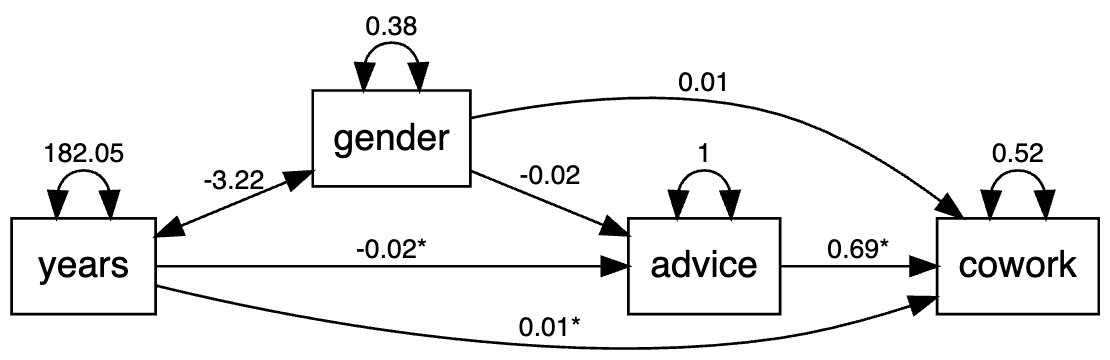
Edge based analysis with latent space model
The R function sem.net.edge.lsm can be used to conduct edge based analysis with latent space model. In this case, the latent distance between each pair of individuals is used along with the transformed non-network covariates in SEM.
Simulated Data Example
To begin with, a random simulated dataset can be used to demonstrate the usage of the node-based network statistics approach. The code below generate a simulated network net with four non-network covariates x1 - x4 which loads on two latent variables lv1, lv2.
set.seed(10)
nsamp = 50
lv1 <- rnorm(nsamp)
net <- ifelse(matrix(rnorm(nsamp^2) , nsamp, nsamp) > 1, 1, 0)
lv2 <- rnorm(nsamp)
nonnet <- data.frame(x1 = lv1*0.5 + rnorm(nsamp),
                     x2 = lv1*0.8 + rnorm(nsamp),
                     x3 = lv2*0.5 + rnorm(nsamp),
                     x4 = lv2*0.8 + rnorm(nsamp))
With the simulated data, we can define a model string with lavaan syntax that specifies the measurement model as well as the relationship between the network and the non-network variables. In this case, we are using net as a mediator between the two latent variables. Since data are generated randomly, the effects should be small overall.
model <-'
  lv1 =~ x1 + x2
  lv2 =~ x3 + x4
  net ~ lv1
  lv2 ~ net
'
Arguments passed to the sem.net.edge.lsm function includes the model, the dataset, and the latent dimensions. Note that data here should be a list with two elements, one being the named list of all network variables and one being the dataframe containing non-network variables. A summary function can be used to look at the output.
data = list(network = list(net = net), nonnetwork = nonnet)
set.seed(100)
res <- sem.net.edge.lsm(model = model, data = data, latent.dim = 1)
summary(res)
path.networksem(res, 'lv2', c('net.dists'), 'lv1')
The output is shown below:
Model Fit InformationSEM Test statistics:  492.628 on 4 df with p-value:  0
network 1 LSM BIC:  2244.546
========================================
========================================

The SEM output:
lavaan 0.6.15 ended normally after 29 iterations

  Estimator                                         ML
  Optimization method                           NLMINB
  Number of model parameters                        11

  Number of observations                          2500

Model Test User Model:

  Test statistic                               492.628
  Degrees of freedom                                 4
  P-value (Chi-square)                           0.000

Model Test Baseline Model:

  Test statistic                               958.550
  Degrees of freedom                                10
  P-value                                        0.000

User Model versus Baseline Model:

  Comparative Fit Index (CFI)                    0.485
  Tucker-Lewis Index (TLI)                      -0.288

Loglikelihood and Information Criteria:

  Loglikelihood user model (H0)             -22209.465
  Loglikelihood unrestricted model (H1)             NA

  Akaike (AIC)                               44440.930
  Bayesian (BIC)                             44504.994
  Sample-size adjusted Bayesian (SABIC)      44470.045

Root Mean Square Error of Approximation:

  RMSEA                                          0.221
  90 Percent confidence interval - lower         0.205
  90 Percent confidence interval - upper         0.238
  P-value H_0: RMSEA <= 0.050                    0.000
  P-value H_0: RMSEA >= 0.080                    1.000

Standardized Root Mean Square Residual:

  SRMR                                           0.109

Parameter Estimates:

  Standard errors                             Standard
  Information                                 Expected
  Information saturated (h1) model          Structured

Latent Variables:
                   Estimate  Std.Err  z-value  P(>|z|)
  lv2 =~
    x4                1.000
    x3                0.976       NA
  lv1 =~
    x2                1.000
    x1                0.642       NA

Regressions:
                   Estimate  Std.Err  z-value  P(>|z|)
  net.dists ~
    lv1              -0.000       NA
  lv2 ~
    net.dists        -0.000       NA

Variances:
                   Estimate  Std.Err  z-value  P(>|z|)
   .x4                2.856       NA
   .x3                1.501       NA
   .x2                1.722       NA
   .x1                2.490       NA
   .net.dists         0.553       NA
   .lv2               1.315       NA
    lv1               0.715       NA

The LSM output:

==========================
Summary of model fit
==========================

Formula:   network::network(data$network[[latent.network[i]]]) ~ euclidean(d = latent.dim)
<environment: 0x7fc473af4960>
Attribute: edges
Model:     Bernoulli
MCMC sample of size 4000, draws are 10 iterations apart, after burnin of 10000 iterations.
Covariate coefficients posterior means:
            Estimate     2.5%   97.5% 2*min(Pr(>0),Pr(<0))
(Intercept) -0.67923 -0.83587 -0.5504            < 2.2e-16 ***
---
Signif. codes:  0 ‘***’ 0.001 ‘**’ 0.01 ‘*’ 0.05 ‘.’ 0.1 ‘ ’ 1

Overall BIC:        2244.546
Likelihood BIC:     2184.507
Latent space/clustering BIC:     60.03918

Covariate coefficients MKL:
             Estimate
(Intercept) -1.117408
Empirical Data Example
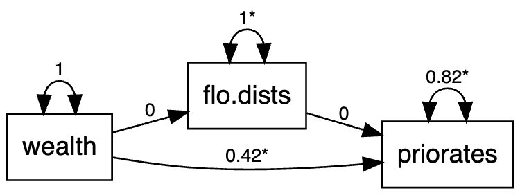
When embedding the LSM into the edge-based approach, one thing that needs to be considered is whether to model covariates predicting the social networks in the LSM framework or in the SEM framework. This is only a concern in the edge-based model since covariates need to be edge-based as well if using the LSM method, and it defies the purpose of simplicity if we consider the LSM in the actor-based approach. In this example, we will accommodate the covariates in the LSM framework within the edge-based approach. The dataset used in this example is the Florentine marriage dataset. The model is quite simple as shown below. Essentially, the observed marriage network is hypothesized to be based not only on the latent positions, but also on the non-network variable of wealth. Additionally, priorates is viewed as a predictor of the distance between latent positrons of the marriage networks.
load("data/flomarriage.RData")

network <- list()
network$flo <- flomarriage.network
nonnetwork <- flomarriage.nonnetwork


model <- '
  flo ~  wealth
  priorates ~ flo + wealth
'
When fitting the model using the sem.net.edge.lsm function, the argument type and latent.dim are needed. Here, although the marriage network contains binary edges, the ordered argument is not needed since only the continuous latent distances will be used in the SEM.
data = list(network=network, nonnetwork=nonnetwork)
set.seed(100)
res <- sem.net.edge.lsm(model=model,data=data, type = "difference", latent.dim = 2, netstats.rescale = T, data.rescale = T)
## results
summary(res)
In this model, the latentnet package is first used to estimate the LSM with the covariate of wealth. Then, the resulting latent positions of the marriage network, taking apart the effect of wealth, is hypothesized to be influenced by priorates and the effect is estimated through lavaan. Thus, the latent distances of the marriage network acts like a mediator between priorates and the observed network. The resulting estimates from both the SEM component and the LSM component are shown below.
Model Fit InformationSEM Test statistics:  0 on 0 df with p-value:  NA
network 1 LSM BIC:  259.7975
========================================
========================================

The SEM output:
lavaan 0.6.15 ended normally after 6 iterations

  Estimator                                         ML
  Optimization method                           NLMINB
  Number of model parameters                         5

  Number of observations                           256

Model Test User Model:

  Test statistic                                 0.000
  Degrees of freedom                                 0

Model Test Baseline Model:

  Test statistic                                50.126
  Degrees of freedom                                 3
  P-value                                        0.000

User Model versus Baseline Model:

  Comparative Fit Index (CFI)                    1.000
  Tucker-Lewis Index (TLI)                       1.000

Loglikelihood and Information Criteria:

  Loglikelihood user model (H0)               -700.431
  Loglikelihood unrestricted model (H1)       -700.431

  Akaike (AIC)                                1410.863
  Bayesian (BIC)                              1428.589
  Sample-size adjusted Bayesian (SABIC)       1412.737

Root Mean Square Error of Approximation:

  RMSEA                                          0.000
  90 Percent confidence interval - lower         0.000
  90 Percent confidence interval - upper         0.000
  P-value H_0: RMSEA <= 0.050                       NA
  P-value H_0: RMSEA >= 0.080                       NA

Standardized Root Mean Square Residual:

  SRMR                                           0.000

Parameter Estimates:

  Standard errors                             Standard
  Information                                 Expected
  Information saturated (h1) model          Structured

Regressions:
                   Estimate  Std.Err  z-value  P(>|z|)
  priorates ~
    wealth            0.422    0.057    7.441    0.000
  flo.dists ~
    wealth            0.000    0.063    0.000    1.000
  priorates ~
    flo.dists        -0.000    0.057   -0.000    1.000

Variances:
                   Estimate  Std.Err  z-value  P(>|z|)
   .priorates         0.819    0.072   11.314    0.000
   .flo.dists         0.996    0.088   11.314    0.000

The LSM output:

==========================
Summary of model fit
==========================

Formula:   network::network(data$network[[latent.network[i]]]) ~ euclidean(d = latent.dim)
<environment: 0x7fc434ed5160>
Attribute: edges
Model:     Bernoulli
MCMC sample of size 4000, draws are 10 iterations apart, after burnin of 10000 iterations.
Covariate coefficients posterior means:
            Estimate   2.5%  97.5% 2*min(Pr(>0),Pr(<0))
(Intercept)   5.0133 2.5627 7.9665            < 2.2e-16 ***
---
Signif. codes:  0 ‘***’ 0.001 ‘**’ 0.01 ‘*’ 0.05 ‘.’ 0.1 ‘ ’ 1

Overall BIC:        259.7975
Likelihood BIC:     85.53086
Latent space/clustering BIC:     174.2666

Covariate coefficients MKL:
            Estimate
(Intercept) 2.861026
To look at indirect effects, the following code can be used.
> path.networksem(res, "wealth","flo.dists", "priorates")
  predictor  mediator   outcome        apath         bpath      indirect
1    wealth flo.dists priorates 2.976241e-21 -4.047181e-22 -1.204539e-42
   indirect_se   indirect_z
1 1.874237e-22 -6.42682e-21
The model is shown in this diagram below.
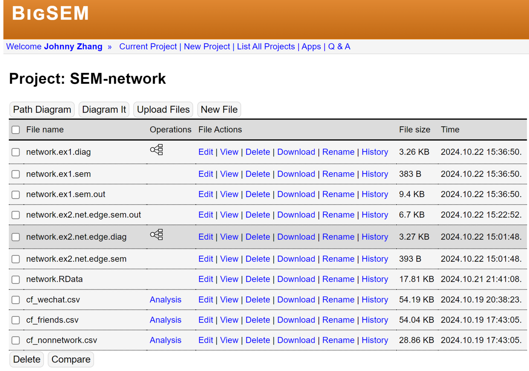
Use of Web App for SEM with Networks
The network data analysis can also be conducted using our online app available at: https://bigsem.psychstat.org/app . To use the app, one need to register as a user to protect the data of the users. Once logging in, a user with work with an interface like below:
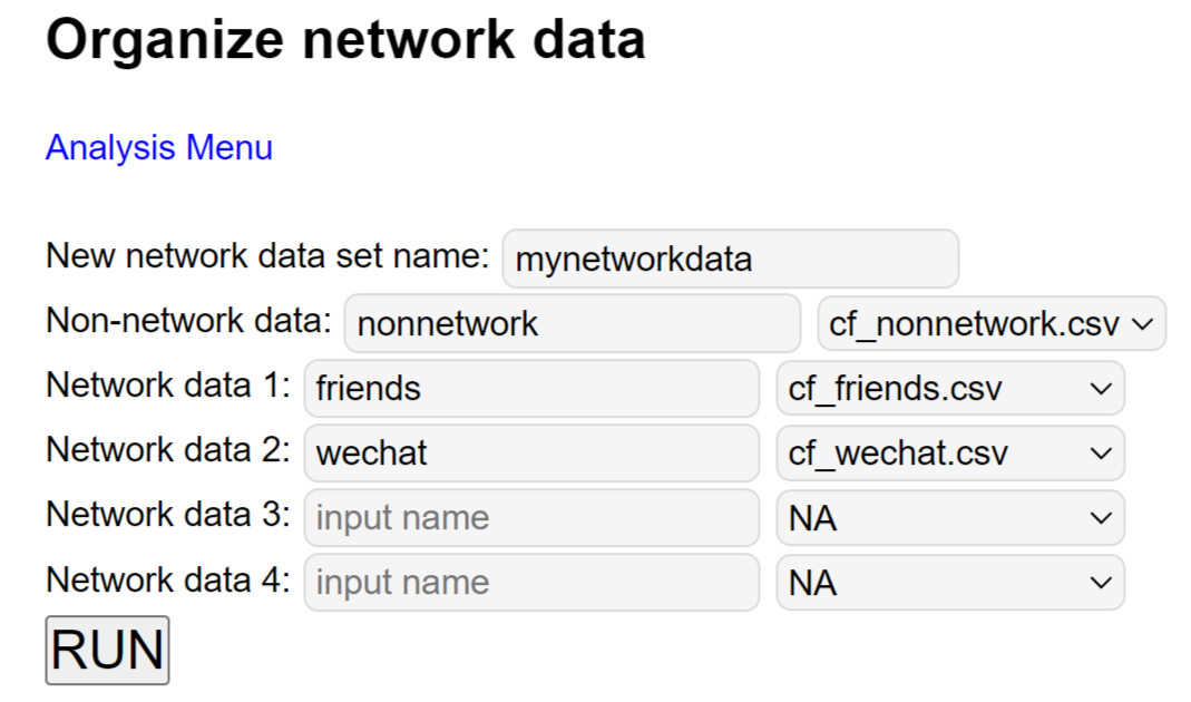
Organizing data
Organizing the data for analysis is the first step for using the app or R package. In R, the data are provided as a list with a non-network component and a network component. To conveniently organize the data online, we developed a simple app.
To use the app, one first upload the non-network data and network data sets as separate files. Then, in the app, one selects the corresponding data files. An example is given below with two networks - friendship and WeChat networks. Note that the new data set will be saved as R data with the provided name, i.e., mynetworkdata.RData in this example.
Conducting the analysis
We use a simple example to illustrate the use of the online app. To conduct the analysis, we need to first draw the path diagram of the model. Here, we create a latent happiness factor (happy.f) from the 4-item measure of global subjective happiness. We then use the friendship network to predict the happiness factor.
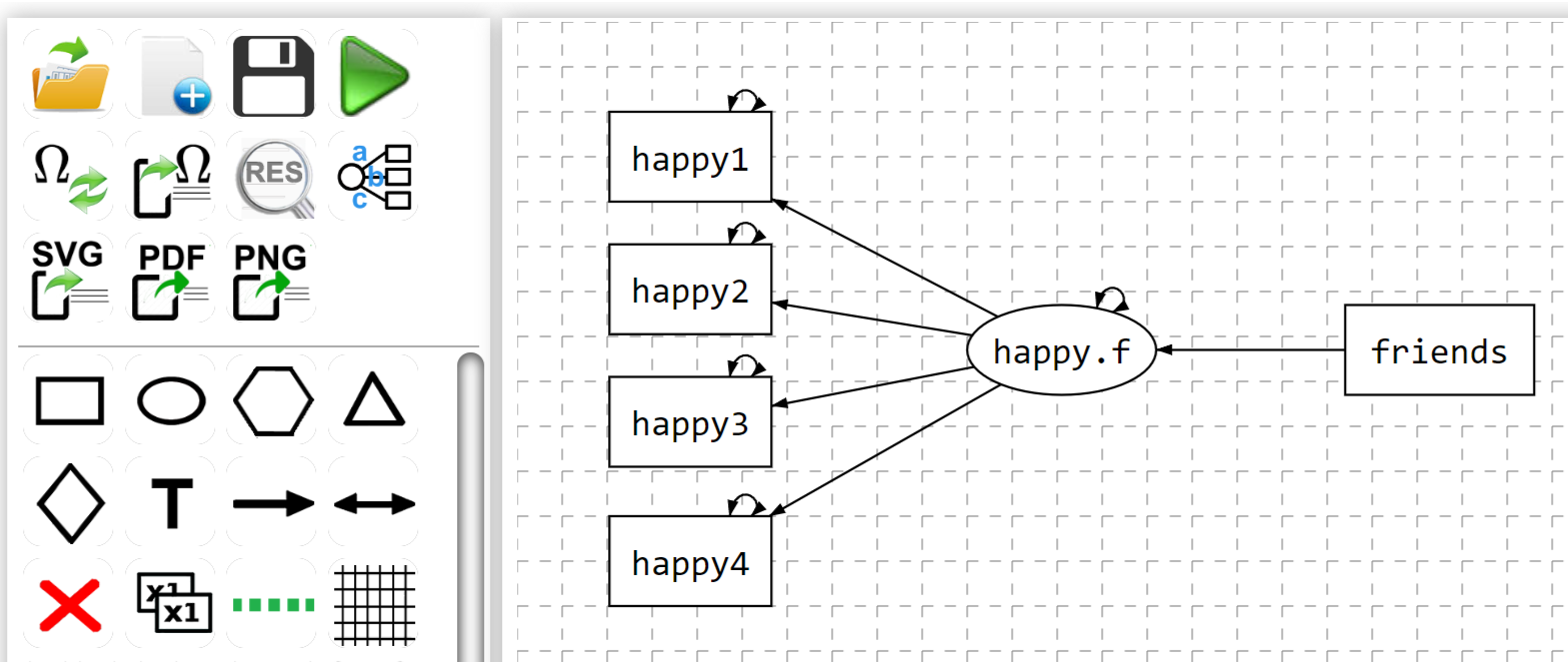
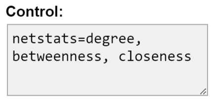
For the network analysis, one needs to choose the software to use, here "NetworkSEM". Then, one selects the Data File "network.RData".
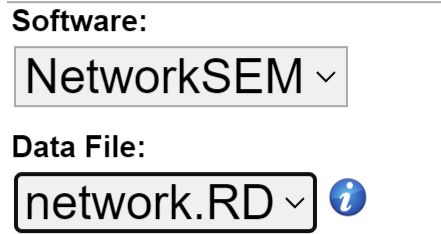
For the network statistics based method, one need to choose what statistics to use. Here, one can specify them in the "Control" field. In this example, we use netstats = degree, betweenness, closeness to allow the use of the three network statistics.
To run the analysis, one clicks on the green triangle in the left panel. The output of the analysis is given below. The output has several parts:
- The basic information, particularly, the user and the analysis id
7cf61d4792351966add082d56368301d. - The descriptive statistics for numerical variables in the non-network data set.
- The information on the networks.
- The basic model information
- The results from fitting the model.
BigSEM started at 15:36:50 on Oct 22, 2024.
=====================================
Please refresh your browser for complete output of complex data analysis.
The current analysis was conducted by the BigSEM user johnny.
To contact us, make sure to include the ticket # for this analysis 7cf61d4792351966add082d56368301d
Descriptive statistics (N=165, p=59)
                   Mean        sd     Min       Max   Skewness Kurtosis
gender          0.55152   0.49885   0.000    1.0000 -0.2071631   1.0429
gpa             3.27293   0.48805   1.173    4.2200 -0.6399076   4.2619
age            21.64242   0.85505  18.000   24.0000 -0.1255522   4.5903
weight         62.29091  14.16756  37.000  110.0000  0.9021334   3.2265
height        169.54545   8.15808 155.000  188.0000  0.3186553   1.9660
smoke           0.26061   0.44030   0.000    1.0000  1.0907192   2.1897
drink           0.41212   0.49372   0.000    1.0000  0.3570735   1.1275
wechat        157.32927 180.36548   0.000 1000.0000  2.9199355  11.9943
id             83.00000  47.77552   1.000  165.0000  0.0000000   1.7999
personality1    2.81818   1.06652   1.000    5.0000 -0.0869982   2.4384
personality2    2.61818   1.22710   1.000    5.0000  0.3212422   2.0339
personality3    2.45455   0.98436   1.000    5.0000  0.4540597   2.8503
personality4    2.64242   0.98743   1.000    5.0000  0.1910639   2.5725
personality5    3.03636   1.15764   1.000    5.0000 -0.0235915   2.2242
personality6    3.07879   1.12612   1.000    5.0000  0.1017642   2.3871
personality7    3.27273   1.16537   1.000    5.0000 -0.1954555   2.1881
personality8    2.36970   1.13816   1.000    5.0000  0.5103888   2.4850
personality9    2.75758   0.94451   1.000    5.0000  0.3684034   3.1224
personality10   3.01212   1.08194   1.000    5.0000  0.0049198   2.5241
personality11   2.89697   1.20276   1.000    5.0000  0.0931915   2.2009
personality12   3.78788   1.08081   1.000    5.0000 -0.4433181   2.2537
personality13   2.61818   1.03283   1.000    5.0000  0.3473757   2.9438
personality14   3.80000   1.04298   1.000    5.0000 -0.5964333   2.8276
personality15   3.42424   1.11613   1.000    5.0000 -0.3898210   2.5711
personality16   2.65455   1.20292   1.000    5.0000  0.2450516   2.2534
personality17   2.31515   0.98033   1.000    5.0000  0.3493841   2.6210
personality18   3.59394   0.99937   1.000    5.0000 -0.1128832   2.1067
personality19   3.82424   0.94966   1.000    5.0000 -0.5435870   3.1673
personality20   3.12121   1.06946   1.000    5.0000  0.0874853   2.4055
depress1        0.98788   0.55202   0.000    3.0000  0.6478164   5.7357
depress2        0.61818   0.58926   0.000    3.0000  0.5205043   3.3723
depress3        0.76364   0.78002   0.000    3.0000  0.8239322   3.2396
depress4        0.91515   0.59884   0.000    3.0000  0.3722678   4.0971
depress5        0.70303   0.67376   0.000    3.0000  0.6728525   3.3429
depress6        0.80606   0.69753   0.000    3.0000  0.7141707   3.7965
depress7        0.66667   0.70998   0.000    3.0000  0.8848909   3.5949
lone1           1.04848   0.77935   0.000    3.0000  0.2260045   2.3813
lone2           1.26667   0.88437   0.000    3.0000  0.1437581   2.2374
lone3           1.03030   0.87251   0.000    3.0000  0.2729773   2.0401
lone4           1.29091   0.90404   0.000    3.0000  0.1403947   2.1952
lone5           1.27879   0.88750   0.000    3.0000  0.0558801   2.1521
lone6           0.85455   0.79828   0.000    3.0000  0.5543989   2.5604
lone7           0.98788   0.85531   0.000    3.0000  0.3749858   2.2210
lone8           1.64242   0.89682   0.000    3.0000 -0.2540419   2.3354
lone9           1.00000   0.86954   0.000    3.0000  0.3907138   2.2320
lone10          0.88485   0.76832   0.000    3.0000  0.5218129   2.7655
happy1          5.34545   1.31897   1.000    7.0000 -0.8142547   3.6334
happy2          5.25455   1.30969   1.000    7.0000 -0.7392627   3.2077
happy3          5.24848   1.30387   2.000    7.0000 -0.4342157   2.6097
happy4          3.89091   1.65654   1.000    7.0000  0.1177261   2.2404
lone            1.12848   0.56674   0.000    2.6000 -0.0868936   2.8135
depress         0.78009   0.41754   0.000    1.8571  0.1401042   2.5266
happy           4.93485   0.86774   2.500    7.0000  0.2112938   3.2653
p.e             2.91364   0.78605   1.000    5.0000  0.1731648   3.4108
p.c             3.53182   0.69743   2.000    5.0000  0.2454618   2.4799
p.i             3.53788   0.68721   1.500    5.0000 -0.2099051   2.6462
p.a             3.55606   0.61259   1.750    5.0000  0.0235716   2.8378
p.n             2.87576   0.63835   1.000    4.7500  0.1728206   3.3815
bmi            21.50942   3.84812  15.401   39.5197  1.5035276   6.1558
              Missing Rate
gender           0.0000000
gpa              0.0000000
age              0.0000000
weight           0.0000000
height           0.0000000
smoke            0.0000000
drink            0.0000000
wechat           0.0060606
id               0.0000000
personality1     0.0000000
personality2     0.0000000
personality3     0.0000000
personality4     0.0000000
personality5     0.0000000
personality6     0.0000000
personality7     0.0000000
personality8     0.0000000
personality9     0.0000000
personality10    0.0000000
personality11    0.0000000
personality12    0.0000000
personality13    0.0000000
personality14    0.0000000
personality15    0.0000000
personality16    0.0000000
personality17    0.0000000
personality18    0.0000000
personality19    0.0000000
personality20    0.0000000
depress1         0.0000000
depress2         0.0000000
depress3         0.0000000
depress4         0.0000000
depress5         0.0000000
depress6         0.0000000
depress7         0.0000000
lone1            0.0000000
lone2            0.0000000
lone3            0.0000000
lone4            0.0000000
lone5            0.0000000
lone6            0.0000000
lone7            0.0000000
lone8            0.0000000
lone9            0.0000000
lone10           0.0000000
happy1           0.0000000
happy2           0.0000000
happy3           0.0000000
happy4           0.0000000
lone             0.0000000
depress          0.0000000
happy            0.0000000
p.e              0.0000000
p.c              0.0000000
p.i              0.0000000
p.a              0.0000000
p.n              0.0000000
bmi              0.0000000
Network data information
        #row #col
friends  165  165
wechat   165  165
Model information
Observed non-network variables: happy1 happy2 happy3 happy4 .
Observed network variables: friends .
Latent variables: happy.f .
The weight is: 0 .
Results
lavaan 0.6-18 ended normally after 66 iterations

  Estimator                                         ML
  Optimization method                           NLMINB
  Number of model parameters                        11

  Number of observations                           165

Model Test User Model:

  Test statistic                                14.749
  Degrees of freedom                                11
  P-value (Chi-square)                           0.194

Model Test Baseline Model:

  Test statistic                               162.858
  Degrees of freedom                                18
  P-value                                        0.000

User Model versus Baseline Model:

  Comparative Fit Index (CFI)                    0.974
  Tucker-Lewis Index (TLI)                       0.958

Loglikelihood and Information Criteria:

  Loglikelihood user model (H0)              -1077.697
  Loglikelihood unrestricted model (H1)      -1070.322

  Akaike (AIC)                                2177.394
  Bayesian (BIC)                              2211.559
  Sample-size adjusted Bayesian (SABIC)       2176.733

Root Mean Square Error of Approximation:

  RMSEA                                          0.045
  90 Percent confidence interval - lower         0.000
  90 Percent confidence interval - upper         0.099
  P-value H_0: RMSEA <= 0.050                    0.498
  P-value H_0: RMSEA >= 0.080                    0.170

Standardized Root Mean Square Residual:

  SRMR                                           0.039

Parameter Estimates:

  Standard errors                             Standard
  Information                                 Expected
  Information saturated (h1) model          Structured

Latent Variables:
                   Estimate  Std.Err  z-value  P(>|z|)
  happy.f =~
    happy4            1.000
    happy3           -4.933    5.032   -0.980    0.327
    happy2           -7.445    7.547   -0.986    0.324
    happy1           -8.133    8.251   -0.986    0.324

Regressions:
                   Estimate  Std.Err  z-value  P(>|z|)
  happy.f ~
    friends.degree   -0.024    0.037   -0.655    0.513
    frinds.btwnnss    0.019    0.029    0.654    0.513
    friends.clsnss    0.011    0.027    0.401    0.689

Variances:
                   Estimate  Std.Err  z-value  P(>|z|)
   .happy4            2.708    0.299    9.070    0.000
   .happy3            1.219    0.147    8.306    0.000
   .happy2            0.633    0.150    4.207    0.000
   .happy1            0.450    0.167    2.701    0.007
   .happy.f           0.019    0.039    0.494    0.621
=====================================
BigSEM ended at 15:36:50 on Oct 22, 2024
BigSEM for Text Data
Text data is increasingly recognized as a rich source of information, offering insights that traditional quantitative measures may overlook. Modern natural language processing (NLP) offers a variety of techniques for analyzing text, such as sentiment analysis (Wankhade et al., 2022), topic modeling (Vayansky & Kumar, 2020), and word embedding (Wang et al., 2019). These techniques automatically extract information from text and transform it into meaningful values or vectors, by-passing the need for labor-intensive manual coding.
Structural equation modeling (SEM) is a popular tool in the social and behavioral sciences for analyzing relationships between observed and latent variables. Incorporating textual data into SEM provides a promising avenue for researchers to integrate qualitative and quantitative data analysis. In response to this opportunity, we developed TextSEM, an R package designed to incorporate text data within SEM frameworks. This package leverages advanced NLP techniques to convert text into quantitative variables, integrate them into SEM model, and conduct estimation.
Here, we demonstrate the practical application of TextSEM through examples using a teaching evaluation dataset.
Example data
For illustration, we use a set of student evaluation of teaching data. The data were scraped from an online website conforming to its site requirement, containing 38,240 teaching evaluations on 1,000 instructors.
For each evaluation, we have information on the overall numerical rating of the teaching of the instructor, how difficult the class was, whether the student took the class for credit or not, grade the student received, etc. The data also contain short textual comments about the instructor's teaching, as well as a list of tabs describing the course. Part of the data are shown below:
'data.frame' : 38240 obs. of  13 variables:
 $ id        : int  1 2 3 4 5 6 7 8 9 10 ...
 $ profid    : int  1 1 1 1 1 1 1 1 1 1 ...
 $ rating    : num  5 5 4 3 1 5 5 2 3 3 ...
 $ difficulty: int  3 4 5 5 5 5 5 4 5 5 ...
 $ credit    : int  1 1 1 1 1 1 1 1 1 1 ...
 $ grade     : int  5 4 5 7 3 NA 6 7 7 8 ...
 $ book      : int  0 0 0 0 0 1 1 1 1 1 ...
 $ take      : int  1 1 1 0 0 0 1 0 NA NA ...
 $ attendance: int  1 1 0 1 1 1 1 1 1 0 ...
 $ tags      : chr  "respected;accessible outside class;skip
                    class? you won't pass ." "accessible outside
                    class;lots of homework;respected" "tough
                    grader;lots of homework;accessible outside
                    class" "tough grader;so many papers;lots of
                    homework" ...
 $ comments  : chr  "best professor i've had in college . only
                    thing i dont like is the writing assignments"
                    "Professor has been the best math professor
                    I've had at thus far . He assigns a heavy
                    amount of homework but "| __truncated__ "He
                    was a great professor . he does give a lot
                    of homework but he will work with you if you
                    don't clearly unders"| __truncated__
                    "Professor is an incredibly respected teacher,
                    however his class is extremely difficult . I
                    believe he just ass"| __truncated__ ...
 $ date      : chr  "04/17/2018" "02/13/2018" "01/07/2018"
                    "12/11/2017" ...
 $ gender    : num  1 1 1 1 1 1 1 1 1 1 ...
The data are included with the R package and can be accessed using
data(prof1000)
Text Sentiment
Sentiment analysis is the process of systematically identifying and quantifying the sentiment expressed in a text.
Lexicon-based / dictionary-based approach
A common method is the lexicon-based approach, where each word is assigned a sentiment score, and the overall sentiment of a sentence is calculated as a weighted average of the words within it. Here, we adopt the approach used by sentimentr (Rinker, 2017), which utilizes a lexicon of polarized words (Hu & Liu, 2004; Jockers, 2017) and adjusts these scores with valence shifters.
The lexicon-based sentiment analysis begins with tokenization, where each paragraph ($p_i$) is broken down into individual sentences ($s_{1}, s_{2}, \cdots,s_{n}$), and each sentence ($s_{j}$) is further decomposed into a sequence of words (${w_{1}, w_{2}, \cdots,w_{m}}$). Thus, each word can be represented as $w_{i, j, k}$. For instance, $w_{2,3,1}$ refers to the first word in the third sentence of the second paragraph.
Next, the words $w_{i, j, k}$ in each sentence are compared against a dictionary of polarized words. Positive words $(w_{i, j, k}^+)$ and negative words $(w_{i, j, k}^-)$ are assigned scores of +1 and -1, respectively. The context surrounding each polarized word is then analyzed, identifying neutral words $(w_{i, j, k}^0)$, negative modifiers $(w_{i, j, k}^n)$, amplifiers $(w_{i, j, k}^a)$, and de-amplifiers $(w_{i, j, k}^d)$. The sentiment score of each word is first weighted by its own score, and then further adjusted based on the function and quantity of valence shifters within its context. The sentiment score of the text is the average sentiment score of all words in the text.
AI-based sentiment analysis
The Korn Ferry Institute's AITMI team made sentiment.ai for researchers and tinkerers who want a straight-forward way to use powerful, open source deep learning models to improve their sentiment analyses. Wiseman et al. (2022) packed the method in an R package sentiment.ai that can produce the sentiment of text and it outperforms many other methods.
The method is based on the Universal Sentence Embedding that embeds a text into a 512 by 1 vector. Then, it build a model between the embedded vector and the labels between the text for prediction.
Online app
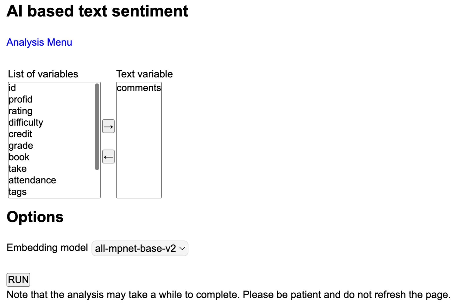
We have developed online apps for both dictionary-based and AI-based sentiment analysis. We created a video to show how to use the AI-based methods to get the sentiment of a text variables. The obtained sentiment score is saved as a new variable in the data set that can be used in further data analysis.
Text Embedding and Encoders
Embedding techniques are widely used in modern NLP. These methods transform text into numerical vectors, capturing both semantic and syntactic relationships with high fidelity (Patil et al., 2023). Conceptually, this process can be viewed as factor analysis or principal component analysis of the text to extract latent information. However, compared to those techniques, embedding vectors are usually of higher dimensionality (e.g., 768 dimensions), which allows for a more detailed representation of semantic and linguistic features.
The evolution of word embedding techniques has been substantial, from basic one-hot encoding to approaches such as Word2Vec, GloVe, and transformer-based models. Notably, transformer models like BERT (Bidirectional Encoder Representations from Transformers) (Devlin et al., 2018) and SentenceBERT (Reimers & Gurevych, 2019) have significantly advanced context-aware sentence embeddings. These models are initially pre-trained on extensive text corpora and can be fine-tuned for specific applications, enhancing their adaptability and effectiveness. BERT utilizes a deep bidirectional transformer architecture to produce contextualized word embeddings that are aggregated into sentence representations. SentenceBERT modifies BERT to optimize it for sentence-level tasks by fine-tuning with natural language inference data, which enhances the ability to compare sentence embeddings via cosine similarity. This optimization boosts BERT’s efficiency
and effectiveness in applications such as semantic similarity assessment and information retrieval.
Furthermore, the development of Large Language Models (LLMs) has improved text embedding generation. OpenAI, for instance, offers several GPT-based embedding models through its API services, including the “text-embedding-3-small” and the more robust “text-embedding-3-large” model (OpenAI, 2024). These models have demonstrated great capabilities across a diverse set of tasks, including semantic search, clustering, and recommendation systems.
TextSEM supports the integration of both SentenceBERT models and OpenAI APIs for generating text embeddings. However, the high dimensionality of these embeddings poses challenges for direct SEM model estimation. To mitigate this, TextSEM employs Principal Component Analysis (PCA) to reduce dimensionality, allowing users to tailor the reduced dimensions to their specific requirements.
Our online app can directly embed text into vectors and save the vectors as an R data set.
Use of the R package TextSEM
The R package TextSEM can be used for SEM analysis with text data. To install the package, please use
## Install the package for text analysis
remotes::install_github("Stan7s/TextSEM")

## The package can be installed from CRAN directly in the future
# install.packages('TextSEM')
We now illustrate the use of the package through several examples.
Sentiment analysis
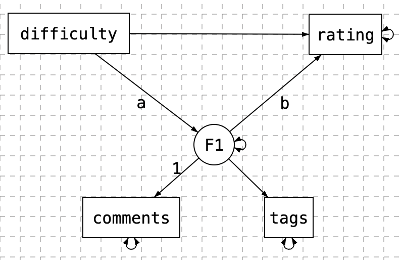
In this example, we introduce how to use the function sem.sentiment to extract sentiment variables from text and estimate the SEM model. Specifically, the overall sentiment of comment is extracted and used as a mediator between three endogenous variables (book, attendance, difficulty) and two exogenous variables (grade and rating).
To use this function, we need to first specify the model:
model <- ' rating ~ book + attendance + difficulty + comments
           grade ~ book + attendance + difficulty + comments
           comments ~ book + attendance + difficulty
         '
The function sem.sentiment requires three parameters: the structural equation model, the input data frame, and the name of the text variable in the data frame to be analyzed for sentiment.
res <- sem.sentiment(model = model,
                     data = prof1000,
                     text_var=c('comments'))
summary(res$estimates, fit = TRUE)
The output of the analysis is given below:
lavaan 0.6.17 ended normally after 63 iterations

  Estimator                                         ML
  Optimization method                           NLMINB
  Number of model parameters                        27

  Number of observations                         38240
  Number of missing patterns                         8

Model Test User Model:

  Test statistic                                 0.000
  Degrees of freedom                                 0

Model Test Baseline Model:

  Test statistic                             31563.154
  Degrees of freedom                                12
  P-value                                        0.000

User Model versus Baseline Model:

  Comparative Fit Index (CFI)                    1.000
  Tucker-Lewis Index (TLI)                       1.000

  Robust Comparative Fit Index (CFI)             1.000
  Robust Tucker-Lewis Index (TLI)                1.000

Loglikelihood and Information Criteria:

  Loglikelihood user model (H0)            -160948.572
  Loglikelihood unrestricted model (H1)    -160948.572

  Akaike (AIC)                              321951.144
  Bayesian (BIC)                            322182.038
  Sample-size adjusted Bayesian (SABIC)     322096.232

Root Mean Square Error of Approximation:

  RMSEA                                          0.000
  90 Percent confidence interval - lower         0.000
  90 Percent confidence interval - upper         0.000
  P-value H_0: RMSEA <= 0.050                       NA
  P-value H_0: RMSEA >= 0.080                       NA

  Robust RMSEA                                   0.000
  90 Percent confidence interval - lower         0.000
  90 Percent confidence interval - upper         0.000
  P-value H_0: Robust RMSEA <= 0.050                NA
  P-value H_0: Robust RMSEA >= 0.080                NA

Standardized Root Mean Square Residual:

  SRMR                                           0.000

Parameter Estimates:

  Standard errors                             Standard
  Information                                 Observed
  Observed information based on                Hessian

Regressions:
                          Estimate  Std.Err  z-value  P(>|z|)
  rating ~
    book                     0.169    0.013   12.905    0.000
    attendance               0.127    0.023    5.618    0.000
    difficulty              -0.331    0.004  -75.262    0.000
    cmmnts.OvrllSn           2.671    0.021  125.974    0.000
  grade ~
    book                    -0.080    0.051   -1.558    0.119
    attendance              -0.170    0.056   -3.058    0.002
    difficulty               0.742    0.020   36.382    0.000
    cmmnts.OvrllSn          -1.756    0.102  -17.171    0.000
  comments.OverallSenti ~
    book                     0.043    0.003   13.053    0.000
    attendance               0.031    0.006    5.290    0.000
    difficulty              -0.074    0.001  -73.666    0.000

Covariances:
                   Estimate  Std.Err  z-value  P(>|z|)
 .rating ~~
   .grade            -0.558    0.024  -23.191    0.000
  book ~~
    attendance        0.017    0.002    8.374    0.000
    difficulty        0.030    0.004    8.650    0.000
  attendance ~~
    difficulty        0.028    0.006    4.712    0.000

Intercepts:
                   Estimate  Std.Err  z-value  P(>|z|)
   .rating            3.995    0.022  182.815    0.000
   .grade             1.807    0.084   21.559    0.000
   .cmmnts.OvrllSn    0.367    0.005   69.455    0.000
    book              0.673    0.003  245.275    0.000
    attendance        0.732    0.004  164.946    0.000
    difficulty        2.928    0.007  445.625    0.000

Variances:
                   Estimate  Std.Err  z-value  P(>|z|)
   .rating            1.034    0.008  136.885    0.000
   .grade             4.222    0.069   61.443    0.000
   .cmmnts.OvrllSn    0.061    0.000  136.529    0.000
    book              0.220    0.002  120.633    0.000
    attendance        0.195    0.003   71.124    0.000
    difficulty        1.651    0.012  138.275    0.000
The path diagram for the model is

Topic modeling
Students' comments about an instructor typically cover multiple topics, such as teaching style, classroom climate, and homework assignments. To identify these topics exploratorily and understand their relationships with other variables, we can apply the sem.topic function. This function performs topic modeling and estimates the SEM model including those identified topics.
In this example, we combine the comments from multiple students for each instructor. We also get the average scores for other variables.
prof.nest <- prof1000 %>% group_by(profid) %>%
summarise(comments = paste(comments, collapse = " "),
          tags = paste(tags, collapse = ";"),
          rating = mean(rating, na.rm = TRUE),
          difficulty=mean(difficulty, na.rm = TRUE),
          book = mean(book, na.rm = TRUE),
          grade=mean(grade, na.rm = TRUE))
In addition to the three required parameters for sem.sentiment – model, data, and text variables, the sem.topic function requires an additional parameter: n_topics. This parameter specifies the number of topics to extract from each column of the text data. Based on previous cross-validation analysis (Jacobucci et al., 2023), six topics were identified in this dataset. Consequently, we will extract six topics. Note that only the first n − 1 topics will be incorporated into the SEM to avoid perfect multicollinearity, where n is the total number of topics specified.
model <- ' rating ~ book + difficulty + comments'
res <- sem.topic(model = model,
                 data = prof.nest,
                 text_var = c('comments'),
                 n_topics = c(6))
summary(res$estimates, fit=TRUE)
The output is given below:
lavaan 0.6.17 ended normally after 1 iteration

  Estimator                                         ML
  Optimization method                           NLMINB
  Number of model parameters                         8

                                                  Used       Total
  Number of observations                           984        1000

Model Test User Model:

  Test statistic                                 0.000
  Degrees of freedom                                 0

Model Test Baseline Model:

  Test statistic                              1143.062
  Degrees of freedom                                 7
  P-value                                        0.000

User Model versus Baseline Model:

  Comparative Fit Index (CFI)                    1.000
  Tucker-Lewis Index (TLI)                       1.000

Loglikelihood and Information Criteria:

  Loglikelihood user model (H0)               -631.624
  Loglikelihood unrestricted model (H1)       -631.624

  Akaike (AIC)                                1279.248
  Bayesian (BIC)                              1318.381
  Sample-size adjusted Bayesian (SABIC)       1292.973

Root Mean Square Error of Approximation:

  RMSEA                                          0.000
  90 Percent confidence interval - lower         0.000
  90 Percent confidence interval - upper         0.000
  P-value H_0: RMSEA <= 0.050                       NA
  P-value H_0: RMSEA >= 0.080                       NA

Standardized Root Mean Square Residual:

  SRMR                                           0.000

Parameter Estimates:

  Standard errors                             Standard
  Information                                 Expected
  Information saturated (h1) model          Structured

Regressions:
                   Estimate  Std.Err  z-value  P(>|z|)
  rating ~
    book              0.295    0.058    5.094    0.000
    difficulty       -0.335    0.023  -14.663    0.000
    comments.topc1    0.392    0.106    3.696    0.000
    comments.topc2    2.503    0.102   24.531    0.000
    comments.topc3    1.637    0.105   15.554    0.000
    comments.topc4   -0.344    0.090   -3.799    0.000
    comments.topc5    0.273    0.093    2.955    0.003

Variances:
                   Estimate  Std.Err  z-value  P(>|z|)
   .rating            0.211    0.010   22.181    0.000
Text embedding
Embedding techniques offer an advantage over topic models in their ability to construct latent factors in higher dimensions from textual data. In this example, we demonstrate how to leverage embedding techniques within the framework of SEM using the sem.emb function.
Before we start, we need to set up the Python environment with the reticulate package, which provides a bridge between R and Python. The code below can be used for the purpose.
library(reticulate)

## First time set-up
virtualenv_create("r-reticulate")
py_install("transformers")
py_install("torch")
py_install("sentence_transformers")
py_install("openai")

## Call virtual environment
use_virtualenv("r-reticulate")
Although it is not required, we recommended first to embed the text and then include the embedded vectors in the SEM analysis .The reason is that text embedding can be time consuming. The embedded data can also be used in multiple models rather than just the model specified.
We can use the sem.encode function to generate text embeddings. This function supports pre-trained models from SentenceBERT and OpenAI. Here, we'll use the all-mpnet-base-v2 model from SentenceBERT. Note that when using OpenAI models, an API key must be specified in the system directory.
embeddings <- sem.encode(prof.nest$comments,
                         encoder = "all-mpnet-base-v2")
## save the embeddings
save(embeddings, file="data/prof.nest.emb.rda")
We then incorporate these embeddings into an SEM model using the sem.emb function. This function allows us to integrate the rich semantic information captured by the embeddings into our statistical model. Two key parameters in this function are: 1) pca_dim: the number of dimensions to retain after applying PCA to the embeddings, and 2) emb_filepath: the file path to the saved embeddings.
sem_model <- ' rating ~ book + difficulty + comments'
res <- sem.emb(sem_model = sem_model,
               data = prof.nest,
               text_var = "comments",
               pca_dim = 10,
               emb_filepath = "data/prof.nest.emb.rda")
The output looks like:
lavaan 0.6.17 ended normally after 1 iteration

  Estimator                                         ML
  Optimization method                           NLMINB
  Number of model parameters                        12

                                                  Used       Total
  Number of observations                           984        1000

Model Test User Model:

  Test statistic                                 0.000
  Degrees of freedom                                 0

Model Test Baseline Model:

  Test statistic                               887.411
  Degrees of freedom                                11
  P-value                                        0.000

User Model versus Baseline Model:

  Comparative Fit Index (CFI)                    1.000
  Tucker-Lewis Index (TLI)                       1.000

Loglikelihood and Information Criteria:

  Loglikelihood user model (H0)               -759.449
  Loglikelihood unrestricted model (H1)       -759.449

  Akaike (AIC)                                1542.898
  Bayesian (BIC)                              1601.598
  Sample-size adjusted Bayesian (SABIC)       1563.486

Root Mean Square Error of Approximation:

  RMSEA                                          0.000
  90 Percent confidence interval - lower         0.000
  90 Percent confidence interval - upper         0.000
  P-value H_0: RMSEA <= 0.050                       NA
  P-value H_0: RMSEA >= 0.080                       NA

Standardized Root Mean Square Residual:

  SRMR                                           0.000

Parameter Estimates:

  Standard errors                             Standard
  Information                                 Expected
  Information saturated (h1) model          Structured

Regressions:
                   Estimate  Std.Err  z-value  P(>|z|)
  rating ~
    book              0.168    0.067    2.517    0.012
    difficulty       -0.406    0.026  -15.524    0.000
    comments.PC1    -10.239    0.549  -18.654    0.000
    comments.PC2     -4.308    0.539   -7.998    0.000
    comments.PC3      7.982    0.573   13.931    0.000
    comments.PC4     -1.373    0.526   -2.612    0.009
    comments.PC5     -0.484    0.534   -0.906    0.365
    comments.PC6      0.034    0.531    0.064    0.949
    comments.PC7      2.664    0.531    5.019    0.000
    comments.PC8     -1.183    0.527   -2.243    0.025
    comments.PC9      0.408    0.531    0.767    0.443

Variances:
                   Estimate  Std.Err  z-value  P(>|z|)
   .rating            0.274    0.012   22.181    0.000
Note that to embed the text and conduct the analysis at the same time, one can use
res <- sem.emb(sem_model = sem_model,
               data = prof.nest,
               text_var = "comments",
               pca_dim = 10,
               encoder = "all-mpnet-base-v2")
Use of Web App
One can conduct the analysis by drawing a path diagram. To start, click the "Path Diagram" button. The interface below will appear:
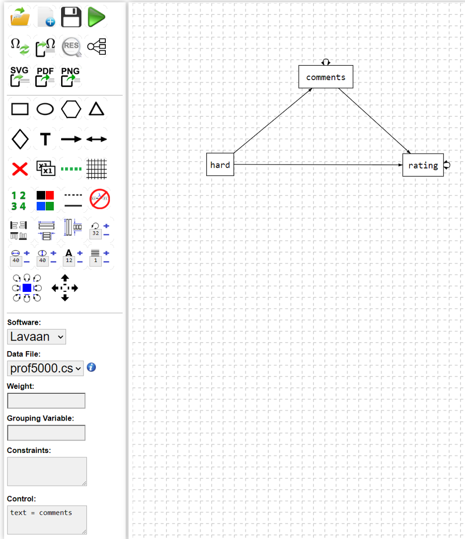
A path diagram can be drawn through the buttons in the interface. In the example, we have a mediation model where the text is used as a mediator for the association of “hard” (how difficulty the class is) and “rating” (the numerical rating of the class).
Different from a regular SEM, we need to specify the variable "comments" as a text variable by setting "text = comments" in the "Control" field. The app also supports different methods including dictionary based sentiment analysis, AI based method (setting "textmethod=ai", and embedding method (setting "textmethod=embedding").
With that, one can click on the run button (the green arrow) to carry out the analysis. For example, for the current model, we have the output as below. It mainly has two parts - the data description and the model results.
Descriptive statistics (N=5000)
                Mean        sd     Min       Max    Skewness Kurtosis
id        1.4343e+04 8314.0453  9.0000 28521.000  5.7205e-03   1.7654
profid    4.8633e+02  299.9069  1.0000  1000.000  2.9661e-02   1.7294
rating    3.8618e+00    1.4581  1.0000     5.000 -9.5170e-01   2.4063
hard      2.8908e+00    1.3156  1.0000     5.000  5.7725e-02   1.8941
sentiment 2.0682e-01    0.2668 -1.4732     1.803 -6.3469e-04   4.6312
          Missing Rate
id                   0
profid               0
rating               0
hard                 0
sentiment            0
Model information
Observed variables: hard comments rating .
Text variables: comments .
The weight is: 0 .
The software to be used is: TextSEM
lavaan 0.6-12 ended normally after 20 iterations

  Estimator                                         ML
  Optimization method                           NLMINB
  Number of model parameters                         9

  Number of observations                          5000
  Number of missing patterns                         1

Model Test User Model:

  Test statistic                                 0.000
  Degrees of freedom                                 0

Model Test Baseline Model:

  Test statistic                              4142.684
  Degrees of freedom                                 3
  P-value                                        0.000

User Model versus Baseline Model:

  Comparative Fit Index (CFI)                    1.000
  Tucker-Lewis Index (TLI)                       1.000

Loglikelihood and Information Criteria:

  Loglikelihood user model (H0)             -15862.021
  Loglikelihood unrestricted model (H1)     -15862.021

  Akaike (AIC)                               31742.042
  Bayesian (BIC)                             31800.696
  Sample-size adjusted Bayesian (BIC)        31772.098

Root Mean Square Error of Approximation:

  RMSEA                                          0.000
  90 Percent confidence interval - lower         0.000
  90 Percent confidence interval - upper         0.000
  P-value RMSEA <= 0.05                             NA

Standardized Root Mean Square Residual:

  SRMR                                           0.000

Parameter Estimates:

  Standard errors                             Standard
  Information                                 Observed
  Observed information based on                Hessian

Regressions:
                          Estimate  Std.Err  z-value  P(>|z|)
  comments.OverallSenti ~
    hard                    -0.075    0.003  -28.208    0.000
  rating ~
    cmmnts.OvrllSn           2.829    0.059   47.785    0.000
    hard                    -0.355    0.012  -29.605    0.000

Intercepts:
                   Estimate  Std.Err  z-value  P(>|z|)
   .cmmnts.OvrllSn    0.424    0.008   50.120    0.000
   .rating            4.304    0.043   99.150    0.000
    hard              2.891    0.019  155.389    0.000

Variances:
                   Estimate  Std.Err  z-value  P(>|z|)
   .cmmnts.OvrllSn    0.061    0.001   50.000    0.000
   .rating            1.076    0.022   50.000    0.000
    hard              1.730    0.035   50.000    0.000
Video tutorials text data analysis
Here we show how to conduct different types of analysis.
Mediation analysis with dictionary-based sentiment
The model used here is
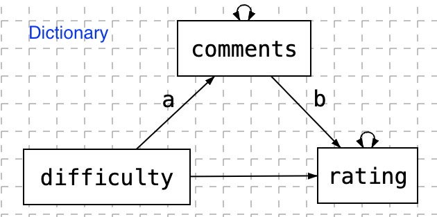
The video tutorial
Mediation analysis with AI-based sentiment
The model is
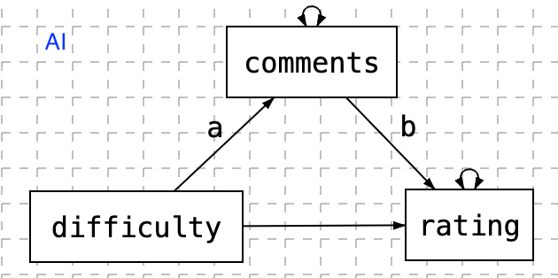
Factor analysis
In this example, we form a factor using two text variables - teaching comments and tags.