Node based analysis with latent space model
The node-based latent space model approach calculates latent positions of the networks, and use them in the SEM analysis along with non-network variables.
Simulated Data Example
To begin with, a random simulated dataset can be used to demonstrate the usage of the node-based network statistics approach. The code below generate a simulated network net with four non-network covariates x1 - x4 which loads on two latent variables lv1, lv2.
set.seed(10)
nsamp = 50
net <- ifelse(matrix(rnorm(nsamp^2), nsamp, nsamp) > 1, 1, 0)
mean(net) # density of simulated network
lv1 <- rnorm(nsamp)
lv2 <- rnorm(nsamp)
nonnet <- data.frame(x1 = lv1*0.5 + rnorm(nsamp),
                     x2 = lv1*0.8 + rnorm(nsamp),
                     x3 = lv2*0.5 + rnorm(nsamp),
                     x4 = lv2*0.8 + rnorm(nsamp))
With the simulated data, we can define a model string with lavaan syntax that specifies the measurement model as well as the relationship between the network and the non-network variables. In this case, we are using net as a mediator between the two latent variables. Since data are generated randomly, the effects should be small overall.
model <-'
  lv1 =~ x1 + x2
  lv2 =~ x3 + x4
  net ~ lv2
  lv1 ~ net + lv2
'
Arguments passed to the sem.net.lsm function includes the model, the dataset, and the number of latent dimensions. Note that data here should be a list with two elements, one being the named list of all network variables and one being the dataframe containing non-network variables. A summary function can be used to look at the output, and the function path.networksem can be used to look at mediation effects across the two latent dimensions.
data = list(network = list(net = net), nonnetwork = nonnet)
set.seed(100)
res <- sem.net.lsm(model = model, data = data, latent.dim = 2)
summary(res)
path.networksem(res, 'lv2', c('net.Z1', 'net.Z2'), 'lv1')
The output looks like the following.
> summary(res)
Model Fit InformationSEM Test statistics:  3.771276 on 6 df with p-value:  0.7075962
NOTE: It is not certain whether it is appropriate to use latentnet's BIC to select latent space dimension, whether or not to include actor-specific random effects, and to compare clustered models with the unclustered model.
network 1 LSM BIC:  2242.696
========================================
========================================

The SEM output:
lavaan 0.6.15 ended normally after 117 iterations

  Estimator                                         ML
  Optimization method                           NLMINB
  Number of model parameters                        15

  Number of observations                            50

Model Test User Model:

  Test statistic                                 3.771
  Degrees of freedom                                 6
  P-value (Chi-square)                           0.708

Model Test Baseline Model:

  Test statistic                                34.438
  Degrees of freedom                                15
  P-value                                        0.003

User Model versus Baseline Model:

  Comparative Fit Index (CFI)                    1.000
  Tucker-Lewis Index (TLI)                       1.287

Loglikelihood and Information Criteria:

  Loglikelihood user model (H0)               -434.447
  Loglikelihood unrestricted model (H1)       -432.561

  Akaike (AIC)                                 898.893
  Bayesian (BIC)                               927.574
  Sample-size adjusted Bayesian (SABIC)        880.491

Root Mean Square Error of Approximation:

  RMSEA                                          0.000
  90 Percent confidence interval - lower         0.000
  90 Percent confidence interval - upper         0.138
  P-value H_0: RMSEA <= 0.050                    0.765
  P-value H_0: RMSEA >= 0.080                    0.165

Standardized Root Mean Square Residual:

  SRMR                                           0.062

Parameter Estimates:

  Standard errors                             Standard
  Information                                 Expected
  Information saturated (h1) model          Structured

Latent Variables:
                   Estimate  Std.Err  z-value  P(>|z|)
  lv2 =~
    x4                1.000
    x3                4.622    6.418    0.720    0.471
  lv1 =~
    x2                1.000
    x1               -0.088    0.271   -0.326    0.744

Regressions:
                   Estimate  Std.Err  z-value  P(>|z|)
  lv1 ~
    lv2              -0.984    0.432   -2.279    0.023
  net.Z1 ~
    lv2              -0.159    0.207   -0.765    0.444
  net.Z2 ~
    lv2               0.208    0.257    0.809    0.418
  lv1 ~
    net.Z1           -0.215    0.169   -1.277    0.202
    net.Z2            0.255    0.138    1.850    0.064

Variances:
                   Estimate  Std.Err  z-value  P(>|z|)
   .x4                1.947    0.425    4.581    0.000
   .x3               -1.587    3.655   -0.434    0.664
   .x2                2.927    6.822    0.429    0.668
   .x1                1.345    0.274    4.906    0.000
   .net.Z1            0.624    0.124    5.012    0.000
   .net.Z2            0.950    0.189    5.013    0.000
    lv2               0.139    0.227    0.612    0.541
   .lv1              -1.984    6.796   -0.292    0.770

The LSM output:

==========================
Summary of model fit
==========================

Formula:   network::network(data$network[[latent.network[i]]]) ~ euclidean(d = latent.dim)
<environment: 0x7fc43202a550>
Attribute: edges
Model:     Bernoulli
MCMC sample of size 4000, draws are 10 iterations apart, after burnin of 10000 iterations.
Covariate coefficients posterior means:
            Estimate     2.5% 97.5% 2*min(Pr(>0),Pr(<0))
(Intercept) -0.18777 -0.42332  0.05               0.1175

Overall BIC:        2242.696
Likelihood BIC:     2107.714
Latent space/clustering BIC:     134.9814

Covariate coefficients MKL:
              Estimate
(Intercept) -0.8639125


> path.networksem(res, 'lv2', c('net.Z1', 'net.Z2'), 'lv1')
  predictor mediator outcome      apath      bpath   indirect
1       lv2   net.Z1     lv1 -0.1587188 -0.2154100 0.03418961
2       lv2   net.Z2     lv1  0.2081154  0.2547222 0.05301162
  indirect_se indirect_z
1  0.04030792  0.8482108
2  0.05368411  0.9874733
Empirical Data Example
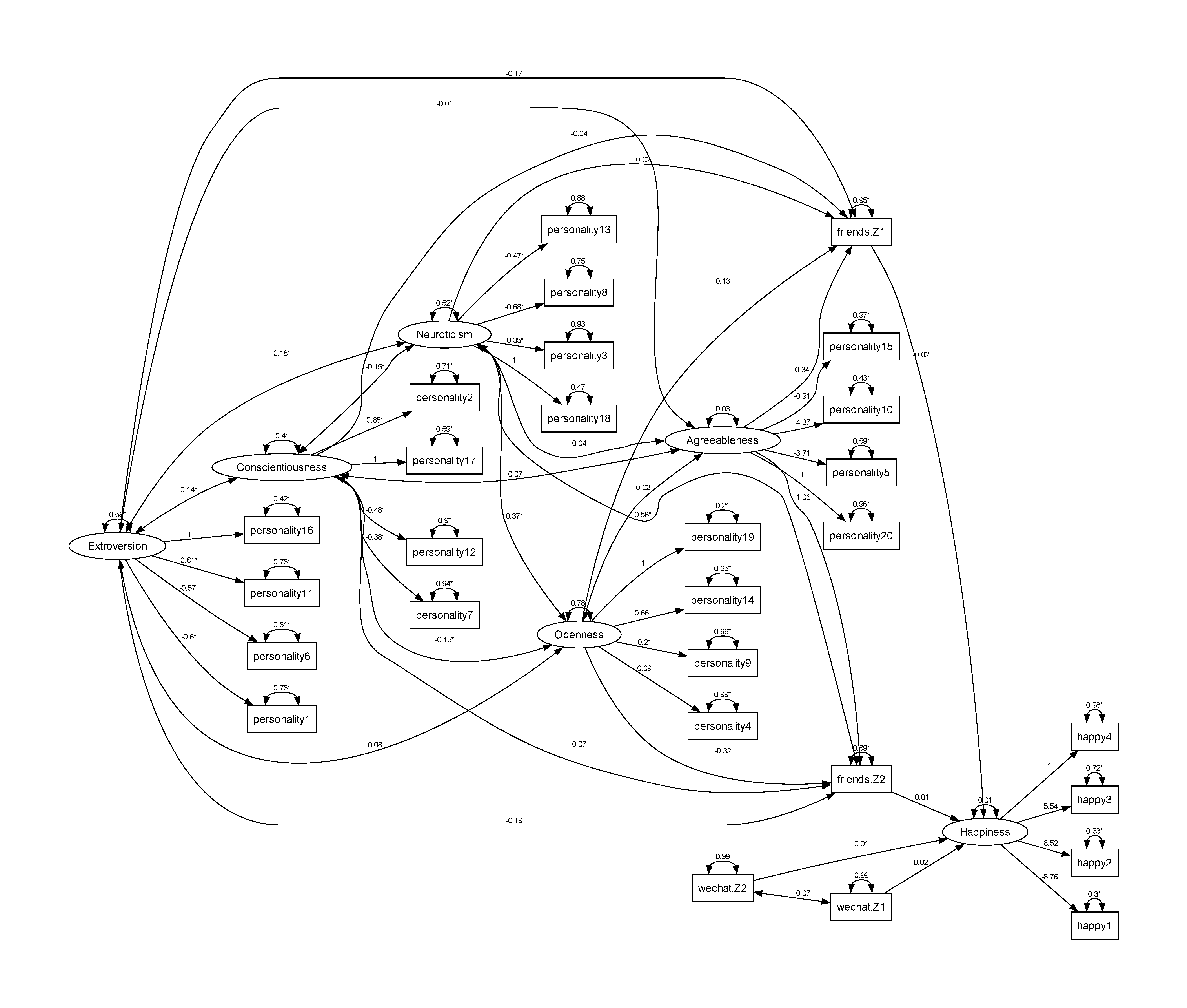
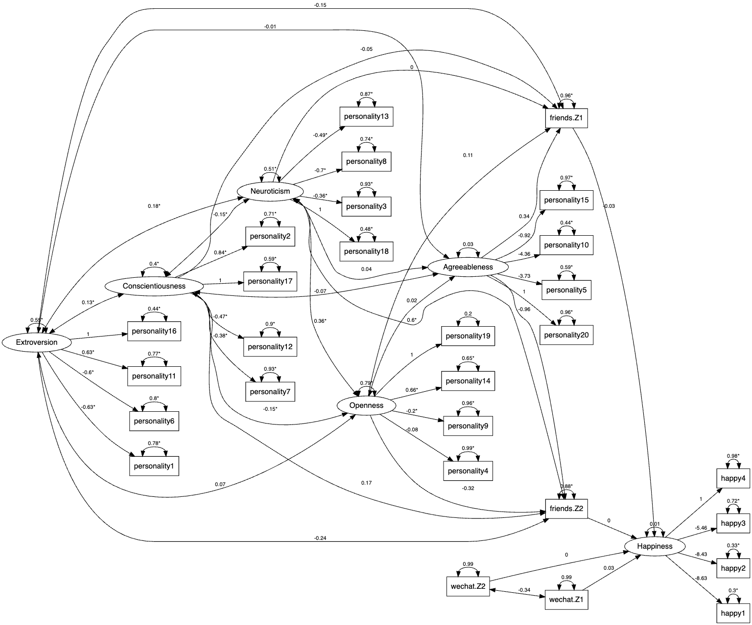
We fit the same model on the friendship and WeChat networks from the network statistics approach using the LSM approach. Under this approach, the latent positions take the roles of the network statistics but the model string can stay the same.
model <-'
  Extroversion =~ personality1 + personality6
                + personality11 + personality16
  Conscientiousness =~ personality2 + personality7
                + personality12 + personality17
  Neuroticism  =~ personality3 + personality8
                + personality13 + personality18
  Openness =~ personality4 + personality9
                + personality14 + personality19
  Agreeableness =~ personality5 + personality10 +
                personality15 + personality20
  Happiness =~ happy1 + happy2 + happy3 + happy4
  friends ~ Extroversion + Conscientiousness + Neuroticism +
  Openness + Agreeableness
  Happiness ~ friends + wechat
'
To fit the model, the sem.net.lsm() function is used. The argument latent.dim should be used to denote the number of latent dimensions to be used in estimating the LSM. A random seed can be set to ensure reproduction of the results, and the argument data.scale = T is used so the scale of the latent positions and the non-network variables are not too different.
data = list(network=network, nonnetwork=non_network)
set.seed(100)
res <- sem.net.lsm(model=model,data=data, latent.dim = 2, data.rescale = T)
For SEM with latent positions, the estimation is again a two-stage process. First, a latent space model with no covariates is used to estimate latent positions through the latentnet R package. The resulting latent positions are then be extracted and compiled into the same dataset as the non-network variables such as the Big Five personality items and the happiness score items, which are then inputted into lavaan to be estimated in the SEM framework. We could again use res$data to access the restructured data with latent positions, and res$model to access the modified model string. The output of sem.net.lsm() has two components in res$estimates - res$estimates$sem.es for lavaan SEM results and res$estimates$lsm.es for latentnet LSM results.
The output of the analysis is given below:
> summary(res)
Model Fit InformationSEM Test statistics:  947.953 on 329 df with p-value:  0
network 1 LSM BIC:  15760.02
network 2 LSM BIC:  15517.77
========================================
========================================

The SEM output:
lavaan 0.6.15 ended normally after 195147 iterations

  Estimator                                         ML
  Optimization method                           NLMINB
  Number of model parameters                        74

  Number of observations                           165

Model Test User Model:

  Test statistic                               947.953
  Degrees of freedom                               329
  P-value (Chi-square)                           0.000

Model Test Baseline Model:

  Test statistic                              1448.277
  Degrees of freedom                               377
  P-value                                        0.000

User Model versus Baseline Model:

  Comparative Fit Index (CFI)                    0.422
  Tucker-Lewis Index (TLI)                       0.338

Loglikelihood and Information Criteria:

  Loglikelihood user model (H0)              -6642.3295824.045
  Loglikelihood unrestricted model (H1)      -6168.3535350.068

  Akaike (AIC)                               13432.65811796.089
  Bayesian (BIC)                             13662.49812025.929
  Sample-size adjusted Bayesian (SABIC)      13428.21411791.645

Root Mean Square Error of Approximation:

  RMSEA                                          0.107
  90 Percent confidence interval - lower         0.099
  90 Percent confidence interval - upper         0.115
  P-value H_0: RMSEA <= 0.050                    0.000
  P-value H_0: RMSEA >= 0.080                    1.000

Standardized Root Mean Square Residual:

  SRMR                                           0.119

Parameter Estimates:

  Standard errors                             Standard
  Information                                 Expected
  Information saturated (h1) model          Structured

Latent Variables:
                       Estimate  Std.Err  z-value  P(>|z|)
  Happiness =~
    happy4                1.000
    happy3               -5.462    4.299    3.529485   -1.218    0.223
    happy2               -8.435    6.668    5.428866   -1.229    0.219
    happy1               -6.8748.634    5.5967.029   -1.229228    0.219
  Agreeableness =~
    personality20         1.000
    personality15        -0.955915    0.754722   -1.267    0.205
    personality10        -4.410359    2.423395   -1.820    0.069
    personality5         -4.0343.726    2.211043   -1.824    0.068
  Openness =~
    personality19         1.000
    personality14         0.722658    0.158144    4.571    0.000
    personality9         -0.200201    0.100   -2.005004    0.045
    personality4         -0.088085    0.101097   -0.873    0.383
  Neuroticism =~
    personality18         1.000
    personality13        -0.508492    0.144139   -3.530529    0.000
    personality8         -0.798701    0.172151   -4.651    0.000
    personality3         -0.354359    0.133135   -2.664    0.008
  Conscientiousness =~
    personality17         1.000
    personality12        -0.523475    0.180163   -2.911    0.004
    personality7         -0.455383    0.189159   -2.412    0.016
    personality2          1.0550.843    0.241193    4.378    0.000
  Extroversion =~
    personality16         1.000
    personality11         0.632    0.151    4.181    0.000
    personality6         -0.559597    0.138148   -4.038    0.000
    personality1         -0.558629    0.134151   -4.170    0.000

Regressions:
                   Estimate  Std.Err  z-value  P(>|z|)
  friends.Z1 ~
    Extroversion     -0.383150    0.457179   -0.838    0.402
  friends.Z2 ~
    Extroversion     -0.586238    0.491199   -1.192    0.233
  friends.Z1 ~
    Conscientisnss   -0.148047    1.0230.327   -0.144    0.885
  friends.Z2 ~
    Conscientisnss    0.503166    1.0480.347    0.480    0.631
  friends.Z1 ~
    Neuroticism      -0.004001    0.718234   -0.006    0.995
  friends.Z2 ~
    Neuroticism       1.7800.600    0.898303    1.982    0.048
  friends.Z1 ~
    Openness          0.352109    0.466144    0.756    0.450
  friends.Z2 ~
    Openness         -1.0030.321    0.559179   -1.794    0.073
  friends.Z1 ~
    Agreeableness     0.961335    2.9301.023    0.328    0.743
  friends.Z2 ~
    Agreeableness    -2.6540.957    3.2601.176   -0.814    0.416
  Happiness ~
    friends.Z1       -0.016029    0.013025   -1.165    0.244
    friends.Z2       -0.002003    0.005009   -0.394    0.693
    wechat.Z1         0.019027    0.017024    1.146    0.252
    wechat.Z2        -0.001002    0.006009   -0.192    0.848

Covariances:
                       Estimate  Std.Err  z-value  P(>|z|)
  Agreeableness ~~
    Openness              0.018    0.019    0.965    0.334
    Neuroticism           0.044041    0.029027    1.538    0.124
    Conscientisnss       -0.075072    0.043041   -1.727    0.084
    Extroversion         -0.011009    0.020015   -0.553    0.580
  Openness ~~
    Neuroticism           0.346365    0.075079    4.596    0.000
    Conscientisnss       -0.141152    0.063068   -2.233    0.026
    Extroversion          0.085074    0.080070    1.063    0.288
  Neuroticism ~~
    Conscientisnss       -0.150153    0.063064   -2.391    0.017
    Extroversion          0.212177    0.081068    2.605    0.009
  Conscientiousness ~~
    Extroversion          0.154130    0.074063    2.073    0.038

Variances:
                   Estimate  Std.Err  z-value  P(>|z|)
   .happy4            2.7020.985    0.298109    9.065    0.000
   .happy3            1.2180.716    0.146086    8.332    0.000
   .happy2            0.569332    0.137080    4.141    0.000
   .happy1            0.522300    0.142082    3.678    0.000
   .personality20     1.1030.965    0.123108    8.968    0.000
   .personality15     1.2080.969    0.134108    8.987    0.000
   .personality10     0.511436    0.135116    3.773    0.000
   .personality5      0.786586    0.135101    5.806    0.000
   .personality19     0.184205    0.139154    1.326    0.185
   .personality14     0.710652    0.107098    6.662    0.000
   .personality9      0.858962    0.095107    9.013    0.000
   .personality4      0.964988    0.106109    9.072    0.000
   .personality18     0.484485    0.104105    4.635    0.000
   .personality13     0.929871    0.109102    8.529    0.000
   .personality8      0.963744    0.125096    7.720    0.000
   .personality3      0.899928    0.102105    8.809    0.000
   .personality17     0.568591    0.102106    5.555    0.000
   .personality12     1.0550.903    0.123105    8.600    0.000
   .personality7      1.2700.935    0.145106    8.781    0.000
   .personality2      1.0650.708    0.151100    7.046    0.000
   .personality16     0.641443    0.167116    3.831    0.000
   .personality11     1.1200.774    0.144099    7.796    0.000
   .personality6      1.0110.797    0.127100    7.983    0.000
   .personality1      0.883776    0.113099    7.813    0.000
   .friends.Z1        9.0340.963    1.0060.107    8.984    0.000
   .friends.Z2        7.7460.881    1.0330.118    7.497    0.000
   .Happiness         0.025009    0.041015    0.615    0.538539
    Agreeableness     0.034029    0.036031    0.934    0.350
    Openness          0.712789    0.168186    4.234    0.000
    Neuroticism       0.508509    0.131    3.880    0.000
    Conscientisnss    0.387403    0.117122    3.310    0.001
    Extroversion      0.798551    0.208143    3.842    0.000

The LSM output:

==========================
Summary of model fit
==========================

Formula:   network::network(data$network[[latent.network[i]]]) ~ euclidean(d = latent.dim)
<environment: 0x7fc412d34470>
Attribute: edges
Model:     Bernoulli
MCMC sample of size 4000, draws are 10 iterations apart, after burnin of 10000 iterations.
Covariate coefficients posterior means:
            Estimate   2.5%  97.5% 2*min(Pr(>0),Pr(<0))
(Intercept)   2.6130 2.5054 2.7225            < 2.2e-16 ***
---
Signif. codes:  0 ‘***’ 0.001 ‘**’ 0.01 ‘*’ 0.05 ‘.’ 0.1 ‘ ’ 1

Overall BIC:        15760.02
Likelihood BIC:     14056.24
Latent space/clustering BIC:     1703.784

Covariate coefficients MKL:
            Estimate
(Intercept) 2.426421


==========================
Summary of model fit
==========================

Formula:   network::network(data$network[[latent.network[i]]]) ~ euclidean(d = latent.dim)
<environment: 0x7fc412d34470>
Attribute: edges
Model:     Bernoulli
MCMC sample of size 4000, draws are 10 iterations apart, after burnin of 10000 iterations.
Covariate coefficients posterior means:
            Estimate   2.5%  97.5% 2*min(Pr(>0),Pr(<0))
(Intercept)   1.1886 1.0938 1.2828            < 2.2e-16 ***
---
Signif. codes:  0 ‘***’ 0.001 ‘**’ 0.01 ‘*’ 0.05 ‘.’ 0.1 ‘ ’ 1

Overall BIC:        15517.77
Likelihood BIC:     13970.87
Latent space/clustering BIC:     1546.901

Covariate coefficients MKL:
            Estimate
(Intercept) 0.967353
The indirect effect from Agreeableness to the latent network positions then to Happiness is given below.
> path.networksem(res,
                  'Agreeableness',
                  c('friends.Z1', 'friends.Z2'),
                  'Happiness')
      predictor   mediator   outcome      apath        bpath
1 Agreeableness friends.Z1 Happiness  0.3354827 -0.028993008
2 Agreeableness friends.Z2 Happiness -0.9573035 -0.003419798
      indirect indirect_se   indirect_z
1 -0.009726651    0.343095 -0.028349729
2  0.003273785    1.125696  0.002908231
The path diagram is givenshown below:as the following.


